The Superposition Principle allows us to determine the overall force exerted on a given charge by any number of point charges. Every charged particle in the universe produces an electric field in the surrounding space. The electric field produced by a charge is unaffected by the presence or absence of additional charges. Coulomb's law can be used to compute the electric field created. The principle of superposition permits two or more electric fields to be combined.
According to the concept of superposition, every charge in space forms an electric field at a place, irrespective of the presence of other charges in that medium. The resulting electric field is a vector sum of the constituent charges' electric fields.
Superposition Principle for Forces Between Multiple Charges
Consider a system in a vacuum with n motionless charges that are stationary: q1, q2, and q3. It has been proven experimentally that the vector sum of all the forces on a charge due to several other charges, taken one at a time, is the vector sum of all the forces on that charge owing to the other charges. Due to the presence of other charges, the separate forces remain unaffected. This is known as the superposition principle.
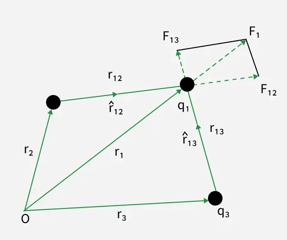
The force on one charge, say q1, due to two other charges, q2 and q3, may be determined by conducting a vector addition of the forces due to each of these charges. As a result, if F12 denotes the force exerted on q1 as a result of q2,
\overrightarrow{F_{12}}=\frac{1}{4\pi\epsilon_0}\frac{q_1q_2}{r^2_{12}}\hat{r}_{12} Similarly, F13 denotes the force exerted on q1 as a result of q3, which again is the Coulomb force on q1 due to q3, even though another charge, q2, is present.
\overrightarrow{F_{13}}=\frac{1}{4\pi\epsilon_0}\frac{q_1q_3}{r^2_{13}}\hat{r}_{13} Thus, the total force F1 on q1 due to the two charges q2 and q3 can be expressed as,
\overrightarrow{F_{1}}=\frac{1}{4\pi\epsilon_0}\frac{q_1q_2}{r^2_{12}}\hat{r}_{12}+\frac{1}{4\pi\epsilon_0}\frac{q_1q_3}{r^2_{13}}\hat{r}_{13}\\ \overrightarrow{F_{1}}=\frac{q_1}{4\pi\epsilon_0}\left[\frac{q_2}{r^2_{12}}\hat{r}_{12}+\frac{q_3}{r^2_{13}}\hat{r}_{13}\right] where
\hat{r_{12}} and\hat{r_{13}} are the unit vectors along the direction of q1 and q2.- ∈o is the permittivity constant for the medium in which the charges are placed.
- r12 and r13 are the distances between the charges.
Continuous Charge Distribution
Dealing with discrete charge combinations involves q1, q2,..., qn. The mathematical treatment is easier and does not require calculus, which is one of the reasons why we limited ourselves to discrete charges. However, working with discrete charges is impractical for many reasons, and we must instead work with continuous charge distributions. All charges are tightly bonded together with very little space between them in a continuous charge distribution.
Charges can be distributed in three ways, including:
- Linear charge distribution
- Surface charge distribution
- Volume charge distribution
1. Linear Charge Density
When charges are dispersed equally along a length, such as around the circumference of a circle or along a straight wire, this is known as linear charge distribution. The units for λ are C/m.
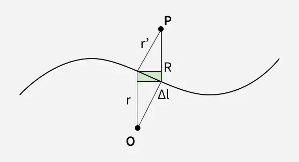
The linear charge distribution is symbolised by the symbol λ. The linear charge density λ of a wire is defined by
Where ∆l is on the macroscopic scale, a small line element of wire, yet it contains a significant number of microscopic charged elements, and ∆Q is the charge contained in that line element.
2. Surface Charge Density
It is impractical to characterise the charge distribution on the surface of a charged conductor in terms of the positions of the tiny charged elements. The unit of surface charge density σ is C/m2.
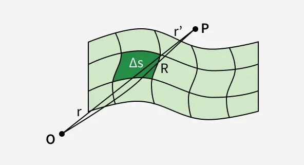
It is more practical to consider an area element S on the conductor's surface (which is small on a macroscopic scale but large enough to contain numerous electrons) and specify the charge Q on that element. A surface charge density σ at the area element by
\sigma=\frac{\Delta{Q}}{\Delta{S}}
The surface charge density σ is a continuous function. The surface charge density, as stated, overlooks charge quantification and charge distribution discontinuities at the microscopic level. , which is a smoothed out average of the microscopic charge density across an area element ∆S, which is huge microscopically but small macroscopically, reflects the macroscopic surface charge density.
3. Volume charge density
When a charge is spread uniformly over a volume, then it is called a volume charge distribution ρ, such as inside a sphere or a cylinder. The unit of volume charge density ρ is C/m3.
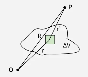
The volume charge density ρ (also known as charge density) is defined.
\rho=\frac{\Delta{Q}}{\Delta{V}}
Where ∆Q denotes the charge in the macroscopically small volume element ∆V, which contains a high number of microscopic charged constituents.
Related Articles:
Sample Questions
Problem 1: A circular annulus of inner radius r and outer radius R has a uniform charge density a.. What will be the total charge on the annulus?
Solution:
The total surface area of the annulus is π×(R2-r2)
It has an outer radius R and an inner radius r.
The surface charge density is the amount of charge stored on the unit surface area.
The surface charge density is a.
Therefore, the total charge on the annulus is π×a×(R2- r2).
Problem 2: What is the dimension of linear charge density?
Solution:
The expression for the Linear charge density λ=(Amount of charge / Total length).
The dimension of electric charge is [I T], and the dimension of length is [L].
Therefore, the dimension of linear-charge-density = [I T L-1].
Problem 3: A charge is distributed along an infinite curved line in space with linear charge distribution λ. What will be the amount of force on a point charge q kept at a certain distance from the line?
Solution:
Let the point charge be situated at a distance r from a small part dl on the line.
The charge stored in stat small part is λ.dl.
The force due to that small part will be directed towards the unit vector
\hat{r} .Therefore, the force on that charge due to the entire linear charge distribution can be written as:
F=q\int\lambda{r^2}\hat{r}dl
Problem 4: A solid nonconducting sphere of radius 1 m carries a total charge of 10 C, which is uniformly distributed throughout the sphere. Determine the charge density of the sphere.
Solution:
The volume of the sphere = (4/3)πr3.
Where r is the radius of the sphere.
Therefore, the charge density, ρ= total charge/[(4/3)πr3].
Now substituting the values,
ρ = 10/[(4/3)πr3]
= 2.38 C/m3.
But if the sphere is conducting, we have to consider the surface charge density.
Problem 5: What is a linear charge distribution?
Solution:
When charges are dispersed equally along a length, such as around the circumference of a circle or along a straight wire, this is known as linear charge distribution. The linear charge distribution is symbolised by the symbol λ. The linear charge density λ of a wire is defined by
\lambda=\frac{\Delta{Q}}{\Delta{l}} Where ∆l is on the macroscopic scale, a small line element of wire, yet it contains a significant number of microscopic charged elements, and ∆Q is the charge contained in that line element.
The units for λ are C/m.