What are State Space Models (SSMs)

A State Space Model (SSM) is a mathematical framework used to model and predict how a system evolves over time. Many real-world systems, such as weather, stock prices or brain signals, change continuously and SSMs help capture these dynamics. The key idea is that each system has hidden internal states that influence the outputs we can see and SSMs learn how these hidden states evolve to make future predictions.

• SSMs separate observable outputs from hidden states.
• They can model systems that change over time and retain memory of the past.
• They handle noise and uncertainty in measurements effectively.
• Linear SSMs use matrices to describe state transitions and observations.

State space is a mathematical representation of a system’s condition at a given time, defined by state variables collected in a state vector, where each point represents a unique system state.

Architecture of State Space Models

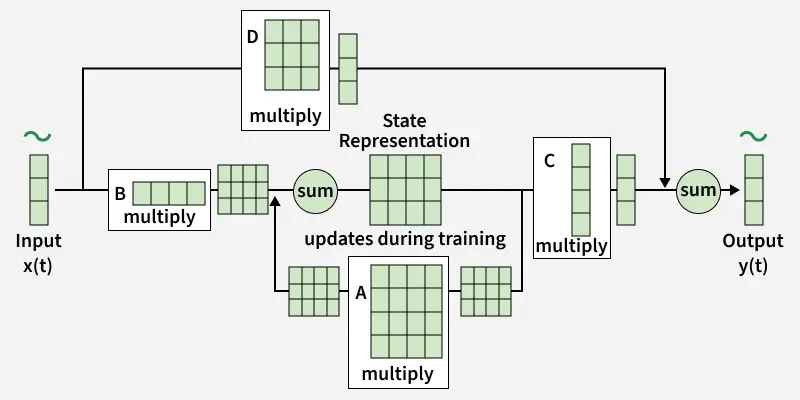
This diagram shows how an SSM processes input by updating a hidden state using matrices A and B, then producing the output through C and D; the model continuously mixes the new input with the evolving state to generate the final output.

• Input x(t) : The external signal or observation fed into the system at time t.
• Matrix B (input-to-state mapping): Transforms the input x(t) into the state space multiplied with x(t) to influence the state update.
• Matrix A (state transition): Represents the dynamics of the system; multiplies the previous state to produce the predicted next state.
• State Representation: The hidden or latent state that evolves over time; updated using contributions from both AAA (previous state) and BBB (current input).
• Matrix D (input-to-output mapping): Directly maps input x(t) to the output without passing through the state, allowing for immediate input effects on output.
• Matrix C (state-to-output mapping): Converts the current state representation into output contributions.
• Sum operations: Combine contributions from state-driven (C × state) and input-driven (D × input) paths to form the final output.
• Output y(t): The observed or predicted signal at time ttt, combining effects from both the current state and direct input.
• Training updates: The state representation is updated during training to minimize prediction error, effectively learning the system dynamics encoded in A, B, C, D.

How Do State Space Models Work

State Space Models (SSMs) describe how systems change over time using a hidden internal state that evolves with each step and generates observable outputs. They track both how the hidden state updates and how it produces the final observations, making them important for modeling dynamic sequential data.

At every time step t:

• Takes an input x(t)
• Updates the hidden state h(t)
• Produces an output y(t) which we can observe

Since the hidden state cannot be seen directly, it is called a latent state.

State Equation

The state equation defines how the hidden internal state of the system evolves over time based on the previous state and the current input.

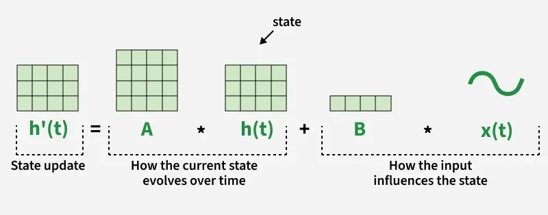
where

• h(t): Hidden state at time t
• h'(t): Updated/next hidden state
• x(t): External input at time t
• A: State transition matrix (controls how the previous state influences the next state)
• B: Input matrix (controls how input affects the state)

Output Equation

The output equation describes how the current hidden state generates the observable output.

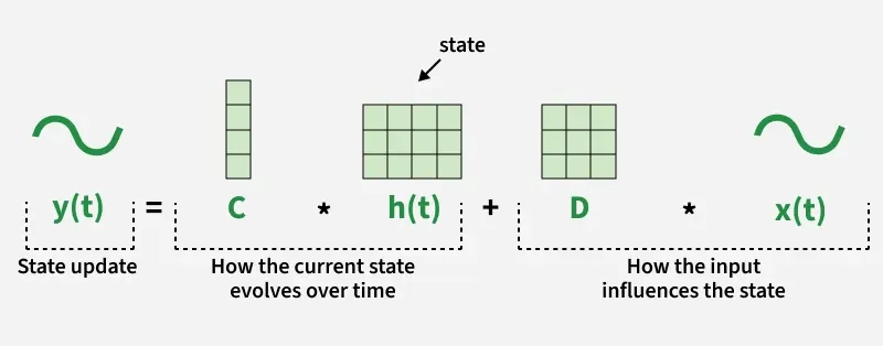
where

• y(t): Output at time t
• C: Output matrix (maps hidden state to output)
• D: Optional feedthrough matrix (direct mapping from input to output)

A, B, C and D define the complete behavior of the system and in machine learning they are typically learned from training data.

Learning SSM Parameters Using Machine Learning

In many real world systems the internal dynamics represented by matrices A, B, C and D are unknown. Machine learning can estimate these parameters from input output data, allowing the SSM to make accurate predictions. For Linear Time Invariant systems methods like Expectation Maximization and Subspace Identification are commonly used.

SSMs in Deep Learning
Deep learning can automatically learn SSM parameters by treating A, B and C as neural network weights:

• The model takes inputs and predicts outputs.
• Predictions are compared with actual outputs using a loss function.
• Backpropagation computes gradients, adjusting A, B and C.
• Gradient descent updates the parameters to minimize loss.

Through training, the model learns the system’s true dynamics without requiring explicit equations.

State Space Models and Their Variants

1. Discrete State Space Models

Traditional SSMs are continuous time models for signals like motion or electrical data but modern deep learning often deals with discrete sequences such as text, clicks or logs. To use SSMs with such data continuous equations are converted to discrete time through discretization, which samples the system at specific time steps.

In discrete form, an SSM behaves like a Recurrent Neural Network (RNN). The latent hidden state of an SSM plays the same role as the hidden state in an RNN.

h_t = \bar{A} h_{t-1} + \bar{B} x_t

y_t = \bar{C} h_t

This equivalence explains why machine learning SSMs often use h for hidden state, similar to RNN notation.

2. Structured State Space Models (S4)

Standard discrete SSMs struggle with long-range dependencies and slow training. S4 addresses these issues using mathematically optimized initialization and fast convolution-based training.

• HiPPO Initialization: HiPPO allows S4 to store long-range sequence information by compressing past inputs into a fixed-size state, preserving important context and improving sequential task performance.
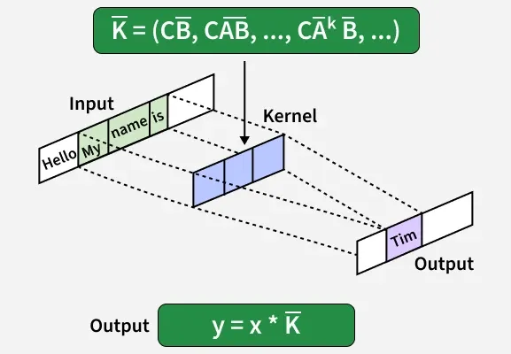
• Connection Between SSMs and CNNs: Discrete SSMs can be converted into 1-D convolution kernels, enabling fast CNN-style training and RNN-style inference, combining the strengths of both architectures.

3. Mamba Models

Mamba is an S6-based model that achieves Transformer-level performance efficiently by selectively attending to important past inputs.

Step By Step Implementation

Here we simulates a time series using a linear state space model, applies a Kalman filter to estimate hidden states and visualizes both the filtered estimates and future predictions.

Step 1: Import Libraries

• Import PyTorch for tensor computation.
• Import Matplotlib for plotting.
• torch.manual_seed() ensures reproducible random outputs.

import torch
from torch import Tensor
from torch.distributions import Normal
import matplotlib.pyplot as plt
import math

torch.manual_seed(42)

Step 2: Define State Transition and Observation Generator

• Implements the SSM state equation and observation equation.
• Matrix F controls how hidden states evolve.
• Vector a maps hidden states to observed values.
• Gaussian noise added to simulate real measurement uncertainty.

def next_obs(current_l: Tensor = torch.tensor([0., 0.]),
             a: Tensor = torch.tensor([1., 1.]),
             F: Tensor = torch.tensor([[1., 1.], [0., 1.]]),
             alpha: float = 0.6, beta: float = 0.6,
             sigma_t: float = 3.0):
 
    g = torch.tensor([alpha, beta])

    y_t = (a * current_l).sum()                      
    obs_noise = sigma_t * torch.randn(1).item()      
    z_t = y_t + obs_noise
    state_noise = torch.randn(1).item()

    next_l = F.matmul(current_l) + g * state_noise
    return next_l, z_t

Step 3: Simulate Synthetic Time-Series

• Uses next_obs() repeatedly to produce observation values.
• Creates noise-based random time-series used later for SSM filtering.

def simulate_single_ts(n_obs: int = 39):
    current_state = torch.tensor([0., 3.])
    obs_list = []
    for _ in range(n_obs):
        current_state, z = next_obs(current_l=current_state)
        obs_list.append(z.item())
    return torch.tensor(obs_list)

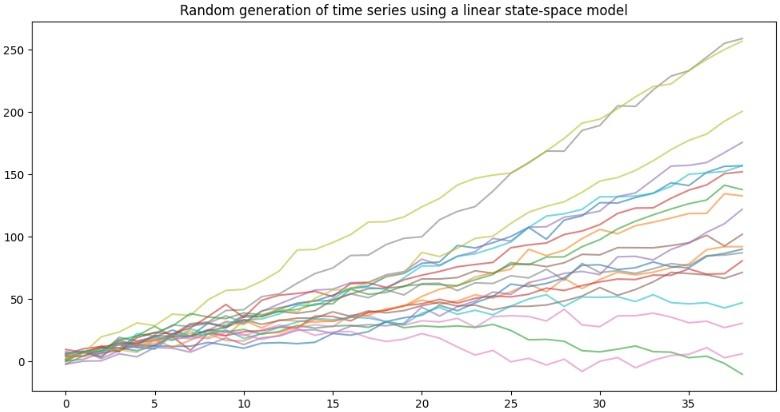
plt.figure(figsize=(12, 6))
for i in range(20):
    plt.plot(simulate_single_ts(), alpha=0.6)
plt.title('Random generation of time series using a linear state-space model')
plt.show()

Output:

Step 4: Build Level-Trend State Space Model Class

• Defines SSM structure using matrices a, F and noise vector g.
• Stores prediction means/variances and hidden state estimate.

class LevelTrendSSM:
   
    a = torch.tensor([1., 1.])                    
    F = torch.tensor([[1., 1.], [0., 1.]])       

    def __init__(self, ts_data: Tensor):
        self.ts_data = ts_data.float()
        self.g = None          
        self.sigma_t = None    
        self.prediction_list = []   
        self.states_list = []      

    @property
    def predictions(self):
        return self.prediction_list

    @property
    def states(self):
        return self.states_list

Step 5: Initialize Kalman Filter Prior

• Sets initial mean f0 and covariance S0.
• Computes first observation estimate.
• Updates using Kalman gain to correct prediction.

def _filter_init(self, alpha: float = 1.0, beta: float = 1.0,
                     sigma_t: float = 3.0,
                     f_0: Tensor = torch.tensor([0., 0.]),
                     S_0: Tensor = torch.diag(torch.tensor([1., 1.]))):
  
        self.g = torch.tensor([alpha, beta])  
        self.sigma_t = float(sigma_t)

        z_mu = (self.a * f_0).sum()
        z_var = (self.a.unsqueeze(0) @ S_0 @ self.a.unsqueeze(1)).item() + (self.sigma_t ** 2)

        residual = self.ts_data[0] - z_mu
        K = (S_0 @ self.a) / z_var
        f_current = f_0 + K * residual

        S_current = S_0 - torch.ger(K, (self.a @ S_0))
        return z_mu, z_var, f_current, S_current

Step 6: Apply Kalman Filtering

• Predict state and covariance for next time step.
• Compute observation mean and variance.
• Update states using observation corrections.

def filter_ts(self, alpha: float = 1.0, beta: float = 1.0,
                  sigma_t: float = 3.0,
                  f_0: Tensor = torch.tensor([0., 0.]),
                  S_0: Tensor = torch.diag(torch.tensor([3., 3.]))):
        self.prediction_list = []
        self.states_list = []
        z_mu, z_var, f_current, S_current = self._filter_init(alpha=alpha, beta=beta,
                                                              sigma_t=sigma_t, f_0=f_0, S_0=S_0)
        self.prediction_list.append([z_mu, z_var])
        self.states_list.append([f_current, S_current])

        for datum in self.ts_data[1:]:
            f_pred = self.F.matmul(f_current)
            S_pred = self.F.matmul(S_current).matmul(self.F.T) + torch.ger(self.g, self.g)

            mu_pred = (self.a * f_pred).sum()
            var_pred = (self.a.unsqueeze(0) @ S_pred @ self.a.unsqueeze(1)).item() + (self.sigma_t ** 2)
            self.prediction_list.append([mu_pred, var_pred])

            residual = datum - mu_pred
            K = (S_pred @ self.a) / var_pred
            f_current = f_pred + K * residual
            S_current = S_pred - torch.ger(K, (self.a @ S_pred))
            self.states_list.append([f_current, S_current])

Step 7: Predict Future Steps

• This function forecasts values beyond the observed sequence.
• Uses the last filtered state from the model to recursively predict future states.
• Computes both mean and variance for uncertainty-aware predictions.
• Returns a list containing predicted values and confidence estimates.

def predict(self, horizon: int):
    assert horizon >= 1
    if not self.states_list:
        raise ValueError('Call filter_ts() first.')
    outputs = []
    f_current, S_current = self.states_list[-1]
    for _ in range(horizon):
        f_current = self.F.matmul(f_current)
        S_current = self.F.matmul(S_current).matmul(self.F.T) + torch.ger(self.g, self.g)
        mu_pred = (self.a * f_current).sum()
        var_pred = (self.a.unsqueeze(0) @ S_current @ self.a.unsqueeze(1)).item() + (self.sigma_t ** 2)
        outputs.append([mu_pred, var_pred])
    return outputs

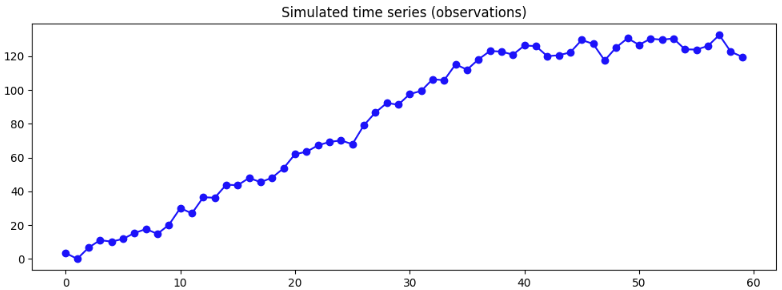
Step 8: Visualize Simulated Observations

• First, plot the raw generated time-series before applying SSM filtering.
• Shows noisy real observations that the model will attempt to smooth and track.
• Useful to visually understand the data the model is working with.

ts_sim = simulate_single_ts(n_obs=60)
plt.figure(figsize=(12, 4))
plt.plot(ts_sim.numpy(), 'bo-', label='Simulated observations')
plt.title('Simulated time series (observations)')
plt.show()

Output:

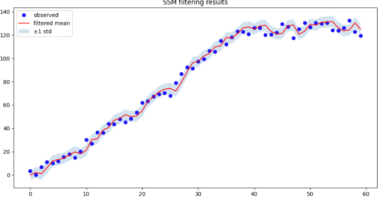
Step 9: Visualize SSM Filtered Results

• Compare original observation points with filtered predicted means from SSM.
• Shaded confidence band shows uncertainty around predictions.
• Helps evaluate how well the SSM smooths noise and tracks trends.

ssm = LevelTrendSSM(ts_sim)
ssm.filter_ts()
preds = ssm.predictions
pred_mus = [p[0] for p in preds]
pred_stds = [math.sqrt(p[1]) for p in preds]

plt.figure(figsize=(12, 6))
plt.plot(ts_sim.numpy(), 'bo', label='observed')
plt.plot(pred_mus, 'r-', label='filtered mean')
plt.fill_between(range(len(pred_mus)),
                 [m - s for m, s in zip(pred_mus, pred_stds)],
                 [m + s for m, s in zip(pred_mus, pred_stds)],
                 alpha=0.2, label='±1 std')
plt.legend()
plt.title('SSM filtering results')
plt.show()

Output:

You can download full code from here

Applications

State Space Models are widely used to model systems that evolve over time and require tracking hidden internal states. They are applied in many real-world fields, including:

• Control Systems: Used in robotics, drones, automotive control and aerospace for stability and trajectory tracking.
• Signal Processing: Filtering noise and estimating true signals (e.g Kalman Filter for radar and GPS tracking).
• Economics and Finance: Forecasting stock markets, inflation rates and economic indicators.
• Weather and Climate Modeling: Predicting temperature, rainfall and climate behavior from sequential data.
• Healthcare ansd Medical Monitoring: Tracking patient vitals and disease progression.
• Speech, Language and Time-Series AI: Used in modern deep learning architectures like S4 and Mamba for long-sequence modeling.

Advantages

• Handles time dependent data efficiently capturing temporal dependencies.
• Classical SSMs are less expressive compared to models with attention mechanisms.
• Can estimate hidden states that are not directly measurable.
• Supports noisy and incomplete data through filtering techniques.
• Scales well for long sequence tasks, especially with structured SSMs like S4 and S6.
• Unifies concepts from RNNs, CNNs anf control theory, enabling flexible machine learning integration.

Limitations of State Space Models

• Difficult to design manually, since parameters (A, B, C, D) must be learned accurately.
• Struggles with very long-range dependencies in basic forms.
• Requires large training data when used with deep learning for parameter learning.
• Neural network based SSMs lose interpretability, making parameters harder to understand.