Regression Analysis with SciPy

Regression analysis is a statistical technique used to examine the relationship between one or more independent variables and a dependent variable. It helps in modelling and analyzing data where the focus is on the relationship between variables. In Python SciPy is a popular library for statistical analysis which offers simple and efficient tools for performing regression using its stats module.

Regression Analysis

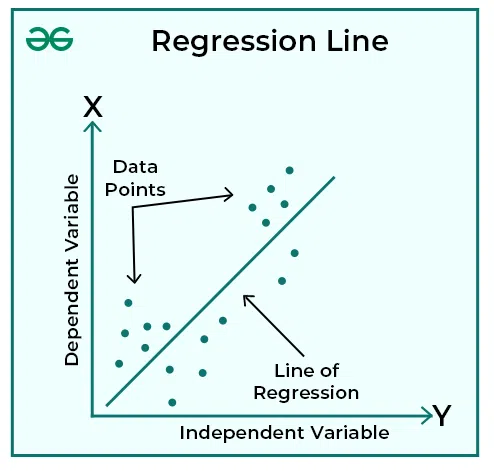
Regression analysis is a statistical technique used to test the relationship between a dependent variable and one or more independent variables. It helps in understanding how the dependent variable changes when any one of the independent variables is varied while the others are held fixed. Regression analysis is commonly used for prediction, forecasting and determining causal relationships between variables.

1. Using SciPy for Linear Regression

Linear Regression models a straight line relationship between one independent and one dependent variable:

y = mx+c

• This code performs Linear regression using SciPy’s linregress() on sample x and y data.
• It calculates the slope, intercept and R squared value to describe the line of best fit.
• Finally, it visualizes the original data points and the fitted regression line using Matplotlib.

import numpy as np
from scipy import stats
import matplotlib.pyplot as plt

# Sample data
x = np.array([1, 2, 3, 4, 5])
y = np.array([2, 4, 5, 4, 5])

# Perform linear regression
slope, intercept, r_value, p_value, std_err = stats.linregress(x, y)

print(f"Slope: {slope}")
print(f"Intercept: {intercept}")
print(f"R-squared: {r_value**2}")

plt.scatter(x, y, color='blue', label='Data')
plt.plot(x, slope * x + intercept, color='red', label='Regression Line')
plt.legend()
plt.xlabel("X")
plt.ylabel("Y")
plt.title("Linear Regression with SciPy")
plt.show()

Output:

2. Using SciPy for Exponential Regression

Exponential Regression is used when data shows exponential growth or decay modelled as:

y = a \cdot e^{bx}

• This code performs Exponential regression using curve_fit from SciPy.
• It fits the data to the model and finds the best values for a and b. The result is plotted by showing both the original data points and the fitted exponential curve.

import numpy as np
from scipy.optimize import curve_fit
import matplotlib.pyplot as plt

#Sample data
x = np.array([0, 1, 2, 3, 4])
y = np.array([1, 2.7, 7.4, 20.1, 54.6])  

# Define the exponential function
def exp_func(x, a, b):
    return a * np.exp(b * x)

# Fit curve
params, _ = curve_fit(exp_func, x, y)
a, b = params
print(f"a = {a}, b = {b}")

# Plot
x_line = np.linspace(min(x), max(x), 100)
plt.scatter(x, y)
plt.plot(x_line, exp_func(x_line, *params), color='green')
plt.show()

Output:

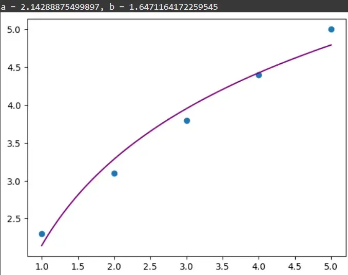
3. Using SciPy for Logarithmic Regression

Logarithmic Regression models relationships where the dependent variable changes proportionally to the logarithm of the independent variable:

y = a + b \ln(x)

• This code fits a Logarithmic regression model to the data using curve_fit. It estimates the parameters a and b that best describe the relationship between x and y.
• The plot visualizes the original data points alongside the fitted logarithmic curve.

import numpy as np
from scipy.optimize import curve_fit
import matplotlib.pyplot as plt

x = np.array([1, 2, 3, 4, 5])
y = np.array([2.3, 3.1, 3.8, 4.4, 5.0])

def log_func(x, a, b):
    return a + b * np.log(x)

params, _ = curve_fit(log_func, x, y)
print(f"a = {params[0]}, b = {params[1]}")

# Plot
x_line = np.linspace(min(x), max(x), 100)
plt.scatter(x, y)
plt.plot(x_line, log_func(x_line, *params), color='purple')
plt.show()

Output:

4. Using SciPy for Logistic Regression

Logistic Regression models S shaped curves often used for classification or growth processes:

y = \frac{L}{1 + e^{-k(x - x_0)}}

• This code fits a Logistic regression curve to the data, modelling an S shaped growth using the logistic function.
• It estimates parameters for curve height (L), growth rate (k) and midpoint (x0) using curve_fit. The plot shows the noisy data points and the smooth fitted logistic curve.

import numpy as np
from scipy.optimize import curve_fit
import matplotlib.pyplot as plt

x = np.linspace(0, 10, 100)
y = 1 / (1 + np.exp(-1.5*(x - 5))) + 0.05 * np.random.normal(size=len(x)) 

def logistic(x, L, k, x0):
    return L / (1 + np.exp(-k*(x - x0)))

params, _ = curve_fit(logistic, x, y, p0=[1, 1, 1])
print(f"L = {params[0]}, k = {params[1]}, x0 = {params[2]}")

plt.scatter(x, y, s=10)
plt.plot(x, logistic(x, *params), color='red')
plt.title("Logistic Regression")
plt.show()

Output: