MAML : Model Agnostic Meta Learning

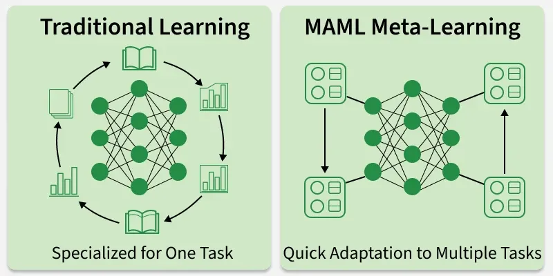
Model-Agnostic Meta-Learning(MAML) is a meta-learning algorithm designed to train models that can adapt to a new task using very few data points and a very few gradient steps, in an essence the model learns to learn.

MAML learns an initialization of parameters/weights such that the model can adapt to any new task in the distribution in relatively fewer steps than random initialization.

Why MAML Exists

In standard training, a model:

• learns one task
• Requires many labelled examples / training data
• Can't generalize well to tasks outside its domain, requires re-training or fine-tuning.

MAML solves this by learning to learn , essentially acting as a effective few-shot learner, MAML shines when

• All the tasks are derived from a single Task distribution (T(x)).
• Each task has very little data.
• Computation is either limited or we want fast adaptations rather than learning from scratch.

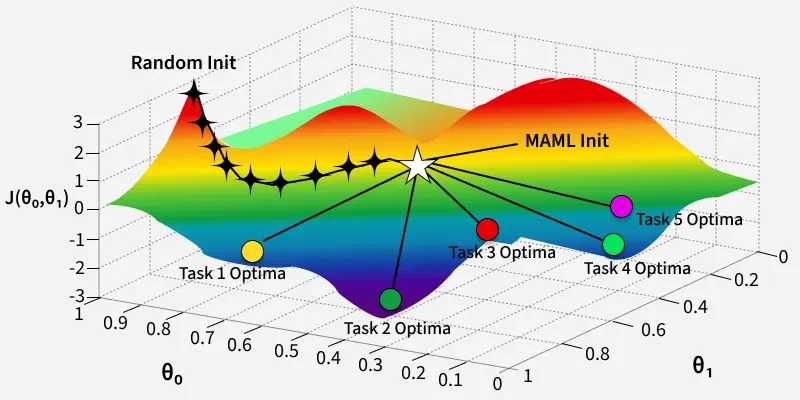
Instead of learning parameters θ that are optimal for one task, MAML learns parameters θ such that, After 1–5 gradient steps on a new task, The adapted parameters perform well on that task. So θ is not the final solution, it is a good starting point.

Algorithm

We will begin with understanding the algorithm mathematically.

Requirements / Hyper-Parameters

p(T) : Probability Distribution from where tasks are sampled
\alpha, \beta : Learning rates for first-order and second-order gradient updates.

Step 1 : Initialize model weights randomly

Model weights are sampled from the uniform distribution
\theta \sim \mu(-a,+a) : where (mu) is a random uniform distribution between +a to -a.

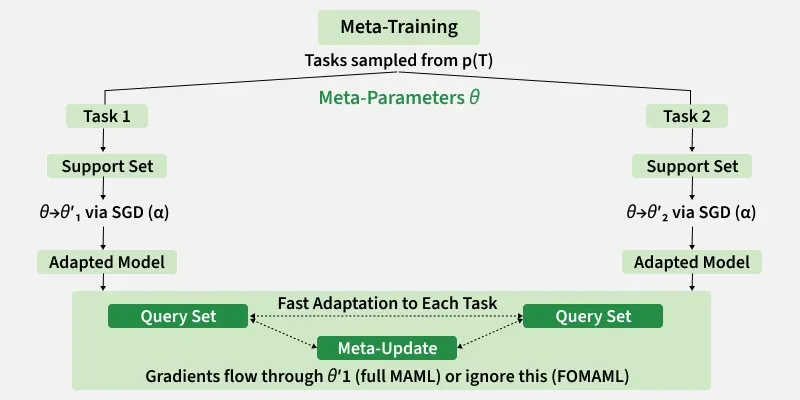
Step 2 : Sampling a Batch of Tasks from the Task distribution

T_i \sim p(T) : One task is sampled from many tasks.

Step 3 : Sample 'K' number of datapoints from the sampled task

\mathcal{D}_i = \{(x^{(i)}, y^{(i)})\} : X is a data point and Y is a label and D_i is the Task's data distribution.

Step 4 : Calculate loss and evaluate gradients

\nabla_{\theta} \mathcal{L}_{\mathcal{T}_i}(f_{\theta}) : where \mathcal{L} is the loss function and \nabla_{\theta} is the gradient w.r.t. loss

Step 5: Compute adapted parameters with gradient descent

\theta_i' = \theta - \alpha \nabla_{\theta} \mathcal{L}_{\mathcal{T}_i}(f_{\theta}) : standard gradient descent update with alpha learning rate

Step 6: Sampled validation data from the task for evaluation

\mathcal{D}_j = \{(x^{(j)}, y^{(j)})\} : This acts as the validation set , sampled from the same task distribution \Rho(\Tau)

Step 7: Calculate gradients like above and update the model parameters

\theta_j' = \theta - \alpha \nabla_{\theta} \mathcal{L}_{\mathcal{T}_i}(f_{\theta}) : Standard gradient update using second-order derivative.

Implementation

Now we will look at implementation of MAML, on a task of predicting family of sine wave functions.

Step 1: Import Necessary Libraries

import numpy as np
import tensorflow as tf

Step 2: Define Task Distribution

Our task distribution will be a family of sine functions with varying amplitude(A) and phase (\phi ) , given by y(t) = A \sin(t + \phi )

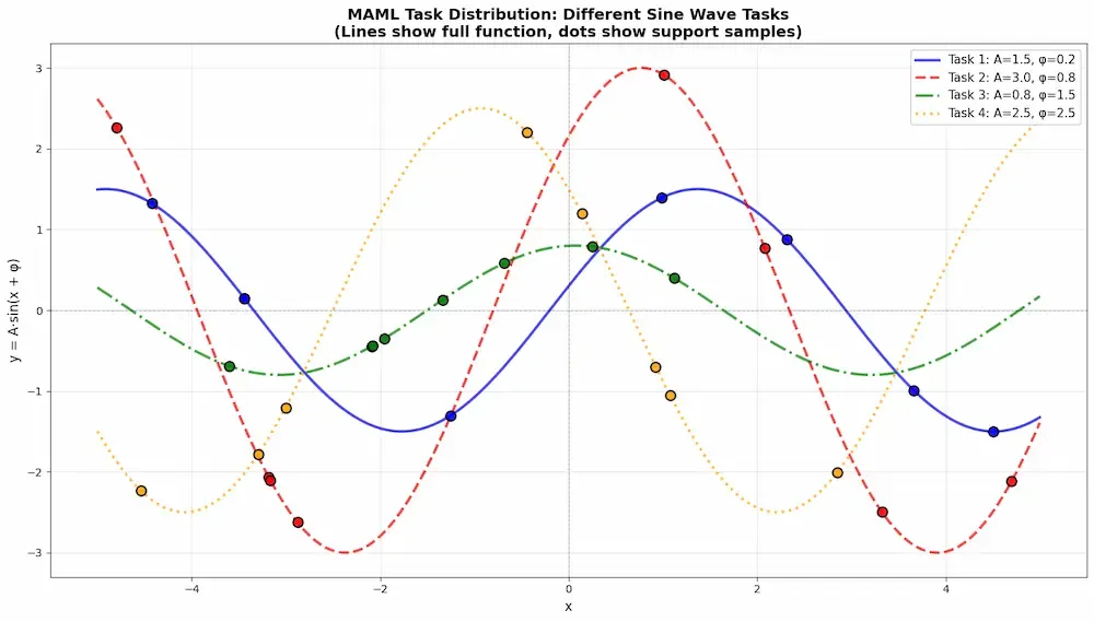
Step 3: Code for Randomly Sampling from the task distribution

• Amplitude(amp) is a uniform distribution over range (0,1 - 5.0)
• phase is also a uniform distribution over 0 to \pi as sinusoidal functions repeat themselves after pi.
• X is the value whose sine will be taken , i.e. sine(x)
• Y is the aggregation of above 3 variables , also we casted the variables into float32 because it's default for tensorflow.

def sample_sine_task(K = 10):
  amp = np.random.uniform(0.1,5.0)
  phase = np.random.uniform(0,np.pi)
  X = np.random.uniform(-5,5,size=(K,1))
  y = amp * np.sin(X + phase)
  return X.astype(np.float32), y.astype(np.float32) # tensorflow default values

Step 4: Define a simple model

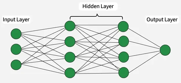
• Model consists of 3 Dense layers with 40 neurons in hidden layer , and 1 in the output layer, with a 'relu' activation function.
• We will be using keras' Sequential API as the flow is sequential in nature.
• we will simulate a forward pass using zero input to build weights.

def create_model():
    return tf.keras.Sequential([
        tf.keras.layers.Dense(40, activation='relu'),
        tf.keras.layers.Dense(40, activation='relu'),
        tf.keras.layers.Dense(1)
    ])

model = create_model()
model(tf.zeros((1, 1))) #dummy forward pass

Output:

Step 5: Define Hyper parameters , loss function and optimizer to use

inner_lr = 0.01 # inner-loop learning rate (alpha)
outer_lr = 0.001 # meta learning rate (beta)
inner_steps = 1 # total iterations of inner
meta_batch_size = 4 # how much batches meta update has

loss_fn = tf.keras.losses.MeanSquaredError()
optimizer = tf.keras.optimizers.Adam(outer_lr)

Step 6: Define a function to simulate forward pass

We will define a function that takes in input and a set of weights and applies a forward pass with those weights, without actually changing the model's weights.

def forward_pass_with_weights(x, weights):
    h = x
    idx = 0

    # layer 1
    h = tf.matmul(h, weights[idx]) + weights[idx + 1]
    h = tf.nn.relu(h)
    idx += 2

    # layer 2
    h = tf.matmul(h, weights[idx]) + weights[idx + 1]
    h = tf.nn.relu(h)
    idx += 2

    # layer 3 (output)
    h = tf.matmul(h, weights[idx]) + weights[idx + 1]

    return h

Step 7: Core MAML training Loop (most important)

• Function first initializes meta_loss to 0 and opens up the outer tf.GradientTape() , which is records operations and performs auto-diff.
• then we sample two datasets one our training set and one is our validation set.
• We record the model's weights , and open up the inner tf.GradientTape()
• After that , we perform a forward pass with these weights , compute the loss , and calculate gradients w.r.t. to the loss.
• we find out and apply the gradients ( Note : The gradients are not applied to the model yet !!)
• We simulate a forward pass with these weights as defined in Step 6 and record the output.
• We increment the meta_loss with the loss between the simulated forward pass and True value.
• Then in the outer loop , we calculate gradient of the gradients , hence performing a double differentiation operation ( this is one of the biggest drawbacks of MAML).
• Then we apply those outer gradients to the model.

@tf.function()
def maml_train_step():
    meta_loss = 0.0
    with tf.GradientTape() as outer_tape:
        for _ in range(meta_batch_size):

            x_train, y_train = sample_sine_task()  # train set
            x_val, y_val = sample_sine_task()      # validation set
            weights = model.trainable_variables    # initial weights

            with tf.GradientTape() as inner_tape:
                y_pred = model(x_train)            # predictions with random variables
                train_loss = loss_fn(y_train, y_pred)  # loss with predictions

            grads = inner_tape.gradient(train_loss, weights)  # gradients with respect to initial loss

            adapted_weights = [
                w - inner_lr * g for w, g in zip(weights, grads)
            ]  # weights ater applying those gradients

            y_val_pred = forward_pass_with_weights(
                x_val, adapted_weights
            )  # if those gradients were applied to the model what would the forward pass output look like

            meta_loss += loss_fn(y_val, y_val_pred)  # meta -loss

        meta_loss /= meta_batch_size

    meta_grads = outer_tape.gradient(
        meta_loss, model.trainable_variables
    )

    optimizer.apply_gradients(
        zip(meta_grads, model.trainable_variables)
    )

    return meta_loss

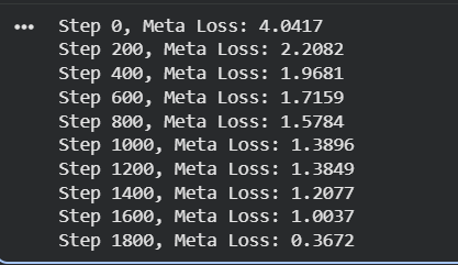
Step 8: Training for 2000 epochs

for step in range(2000):
    loss = maml_train_step()
    if step % 200 == 0:
        print(f"Step {step}, Meta Loss: {loss.numpy():.4f}")

Output:

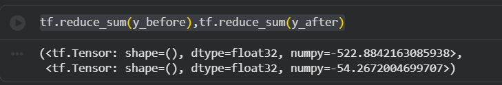
Step 9: Evaluating the model on unseen task for one-step adaption:

Now we check the performance of a model that has not seen the task before v/s after MAML optimized model.

# New unseen task
x_train, y_train = sample_sine_task()
x_test = np.linspace(-5, 5, 100).reshape(-1, 1).astype(np.float32)

# Before adaptation
y_before = model(x_test)

# One-step adaptation
with tf.GradientTape() as tape:
    loss = loss_fn(y_train, model(x_train))
grads = tape.gradient(loss, model.trainable_variables)

adapted_weights = [
    w - inner_lr * g for w, g in zip(model.trainable_variables, grads)
]

y_after = forward_pass_with_weights(x_test, adapted_weights)
print(tf.reduce_sum(y_before),tf.reduce_sum(y_after))

Output:

You can find and download the updated code from here.

Applications of MAML

1. Few-shot image Classification : MAML demonstrates that few-shot learning can be framed as a meta-learning problem , MAML has demonstrated exception performance on datasets like Mini-Image-Net and Omniglot , making it a competitive baseline for few-shot tasks.
2. Robotics : Robots have to interact with environment and make quick decisions based on limited data and limited time , MAML shines here by optimizing for quick decision-making under less external data.
3. Reinforcement Learning : MAML accelerates policy adaption in neural networks by initializing neural networks policies to regions of parameter space where task-specific policies can be learned quickly via gradient descent.

Limitations

1. Computational complexity and memory overhead : MAML requires second-order derivatives through the inner loop updates, making it computationally expensive. This results in higher memory consumption and training times that can be 2x or 3x longer than first-order alternatives.
2. Training Instability : As MAML is a bi-optimization problem , small changes to hyper-parameters can lead to poor training.
3. Question of Objective : Yes, MAML optimizes to optimizes but in some cases this makes things worse than improve , MAML usually settles in areas where gradients are accessible easily , but normal first-order derivatives , can reach there in a few iterations near easily, making MAML unnecessary.