Expected value and variance are fundamental concepts in probability and statistics that help us understand the behavior of random variables. The expected value, also known as the mean, represents the average outcome of an experiment repeated many times. Variance, on the other hand, measures the spread or dispersion of a set of values.
For example, if you were to roll a fair six-sided die, the expected value of the roll would be the average of all possible outcomes; meanwhile, the variance would give you an idea of how much each roll deviates from this average value.
In this article, we will discuss Expected Value and Variance in detail.
Expected Value
The expected value (often denoted as E(X) or μ) of a random variable X is a measure of the central tendency of its probability distribution. It is essentially the mean value that the variable would take if the experiment were repeated many times.
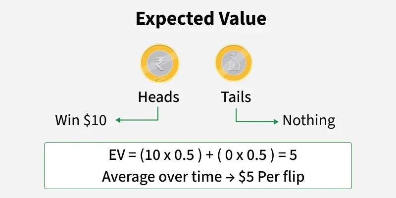
In Figure 1, we can understand the concept of expected value:
You play a game where:
- You win ₹10 if you get Heads
- You win ₹0 if you get Tails
The coin is fair (so the probability of Heads = 0.5 and Tails = 0.5).
If you play this game many times, you’ll win ₹5 on average per flip — even though you never actually win exactly ₹5 in any single flip. That's the expected value.
Expected value can be thought of as the "center of mass" of the probability distribution. It is the point at which the distribution would balance if it were possible to place it on a scale.
Formula for Expected Value
The expected value of a discrete random variable X with possible values x1, x2,..., xn and corresponding probabilities p1, p2,...,pn is given by:
E(X) = \sum_{i=1}^{n} x_i \cdot p_i
For a continuous random variable X with probability density function f(x), the expected value is defined as:
E(X) = \int_{-\infty}^{\infty} x \cdot f(x) \, dx
Example 1: Find the expected value when rolling a fair six-sided die.
Solution:
Possible outcomes: 1, 2, 3, 4, 5, 6
Probabilities: P(X=i) =
\frac{1}{6} for i = 1,...,6Expected value calculation:
E(X) = \sum_{i=1}^{6} x_i \cdot P(X=x_i) \\E(X)= 1 \cdot \frac{1}{6} + 2 \cdot \frac{1}{6} + 3 \cdot \frac{1}{6} + 4 \cdot \frac{1}{6} + 5 \cdot \frac{1}{6} + 6 \cdot \frac{1}{6} \\E(X) = \frac{1+2+3+4+5+6}{6} = \frac{21}{6} = 3. 5 The expected value of a fair die roll is 3.5.
Example 2: Find the expected waiting time when the time is uniformly distributed between 0 and 10 minutes.
Solution:
Probability density function (PDF):
f(x) = \begin{cases} \frac{1}{10} & \text{for } 0 \leq x \leq 10 \\ 0 & \text{otherwise} \end{cases} Expected value calculation:
E(X) = \int_{-\infty}^{\infty} x \cdot f(x) \, dx = \int_{0}^{10} x \cdot \frac{1}{10} \, dx \\ E(X) = \frac{1}{10} \int_{0}^{10} x \, dx = \frac{1}{10} \left[ \frac{x^2}{2} \right]_0^{10} \\ E(X) = \frac{1}{10} \cdot \frac{100}{2} = 5 The expected waiting time is 5 minutes.
Properties of Expected Value
Some of the properties of expected value are listed in the following table:
| Property | Description | Formula | Example |
|---|---|---|---|
| Linearity of Expectation | The expected value of a linear combination of random variables is the linear combination of their expectations. | E(aX + bY) = aE(X) + bE(Y) | If E(X) = 2 and E(Y) = 3, then E(2X + 3Y) = 2⋅2 + 3⋅3 = 13 |
| Expected Value of a Constant | The expected value of a constant is the constant itself. | E(c) = c | If c=5, then E(5) = 5. |
| Sum of Random Variables | The expected value of the sum of random variables is the sum of their expected values. | E(X + Y) = E(X) + E(Y) | If E(X) = 2 and E(Y) = 3, then E(X + Y) = 2 + 3 = 5 |
| Product of a Constant and a Random Variable | The expected value of a constant multiplied by a random variable is the constant multiplied by the expected value of the variable. | E(aX) = aE(X) | If a = 4 and E(X) = 2, then E(4X) = 4⋅2 = 8 |
| Non-Negativity for Non-Negative Random Variables | The expected value of a non-negative random variable is non-negative. | E(X) ≥ 0 if X ≥ 0 | If X ≥ 0, then E(X) ≥ 0. |
| Expectation and Independence | For independent random variables, the expected value of their product is the product of their expected values. | E(XY) = E(X) ⋅ E(Y) | If X and Y are independent, E(X) = 2 and E(Y) = 3, then E(XY) = 6 |
| Indicator Variables | The expected value of an indicator variable equals the probability of the event it indicates. | E(IA)=P(A) | If P(A) = 0.7, then E(IA) = 0.7 |
| Jensen's Inequality | For a convex function g, the expected value of g(X) is at least g of the expected value of X. | E(g(X)) ≥ g(E(X)) | For a convex g, E(g(X)) ≥ g(E(X)). |
Variance
Variance is a statistical measure that indicates the spread or dispersion of a set of data points. It shows how much the data points in a dataset differ from the mean (average) value.
A high variance indicates that the data points are spread out widely around the mean, while a low variance indicates that they are clustered closely around the mean. Variance helps in understanding the variability within a dataset.
In real-world applications, variance is used in finance to assess risk, in quality control to measure consistency, and in many other fields to analyze variability.
Formula for Variance
Population Variance (σ²)
The formula for the variance of a population is:
\sigma^2 = \frac{\sum_{i=1}^{N} (x_i - \mu)^2}{N}
Where:
- σ2 is the population variance.
- xi represents each data point in the population.
- μ is the mean of the population.
- N is the total number of data points in the population.
Sample Variance (s²)
The formula for the variance of a sample is:
s^2 = \frac{\sum_{i=1}^{n} (x_i - \bar{x})^2}{n-1}
Where:
- s2 is the sample variance.
- xi represents each data point in the sample.
\bar{x} is the mean of the sample.- n is the total number of data points in the sample.
Example: Find the population variance for outcomes of a fair six-sided die.
Solution:
Possible outcomes: X in 1, 2, 3, 4, 5, 6
Probabilities:P(X=i) = \frac{1}{6} \: for \: i = 1,\ldots,6
Mean (from previous): = 3.5
\sigma^2 = \frac{\sum_{i=1}^{6} (x_i - \mu)^2}{6} \\ \sigma^2 = \frac{(1-3.5)^2 + (2-3.5)^2 + \cdots + (6-3.5)^2}{6} \\ \sigma^2 = \frac{6.25 + 2.25 + 0.25 + 0.25 + 2.25 + 6.25}{6} \\ \sigma^2 = \frac{17.5}{6} \approx 2.9167 The population variance of a fair die is
{\dfrac{35}{12}} (exact) or 2.9167 (approximate).
Relationship Between Expected Value and Variance
Variance can also be expressed using the expected value in the following way:
Var(X) = E[(X − E(X))2]
This formula can be expanded to show the relationship between the expected value and variance more explicitly:
Var(X) = E[(X − E(X))2] = E[X2 − 2XE(X) + (E(X))2]
Using the linearity of expectation, this becomes:
Var(X) = E[X2] − 2E(X)E(X)+(E(X))2 = E[X2] − (E(X))2
Therefore, the variance of a random variable X can be calculated as the difference between the expected value of the square of X and the square of the expected value of X:
Var(X) = E[X2]−(E(X))2
Example: A casino game uses a special 4-sided die with the following probability distribution: for outcomes 1, 2, 3, and 4, the probabilities are 0.1, 0.4, 0.3, and 0.2, respectively. Find the variance of the payout.
Solution:
E[X] = \sum x_i P(x_i) \\ E[X] = (1)(0.1) + (2)(0.4) + (3)(0.3) + (4)(0.2) \\ E[X] = 0.1 + 0.8 + 0.9 + 0.8 = 2.6 E[X^2]= \sum x_i^2 P(x_i) \\ E[X^2]= (1^2)(0.1) + (2^2)(0.4) + (3^2)(0.3) + (4^2)(0.2) \\ E[X^2]= (1)(0.1) + (4)(0.4) + (9)(0.3) + (16)(0.2) \\ E[X^2]= 0.1 + 1.6 + 2.7 + 3.2 = 7.6 Var(X) = E[X^2] - (E[X])^2 \\ Var(X) = 7.6 - (2.6)^2 \\ Var(X) = 7.6 - 6.76 \\ Var(X) = 0.84
Applications of Expected Values and Variance
In computer science, especially in areas like algorithm analysis, machine learning, and data analysis, expected value and variance are the fundamental concepts with practical significance:
- Algorithm Analysis: Analyzing the expected running time or output of an algorithm, especially randomized algorithms.
- Machine learning: Evaluating model performance, optimizing algorithms (e.g., reinforcement learning to maximize expected rewards), making predictions using probabilistic models, and selecting the best model based on metrics like expected accuracy or loss.
- Data Analysis: Summarizing datasets using expected values to estimate population means.
- Gaming & Gambling: Used to determine the probability of winning or losing in games of chance, helping players and casinos make informed decisions.
- Bias-Variance Tradeoff: In machine learning, variance is crucial in understanding the bias-variance tradeoff – a fundamental concept balancing model complexity and generalization capability.