DBScan (Density-Based Spatial Clustering of Applications with Noise) is a non-linear, unsupervised clustering algorithm that identifies groups (clusters) of densely packed data points without requiring the number of clusters to be specified beforehand. Unlike algorithms like k-means, DBScan is capable of discovering arbitrarily shaped clusters and distinguishing noise or outliers in datasets.
How Does DBSCAN Work?
- Choose the parameters eps (neighborhood radius) and MinPts (minimum points to form a dense region).
- Select an unvisited point and find all neighboring points within the eps radius.
- If the number of neighbors is at least MinPts, classify it as a core point and start a new cluster.
- Expand the cluster by including all density-reachable points connected to the core point.
- Repeat the process for all unvisited points until every point is assigned to a cluster or marked as noise.
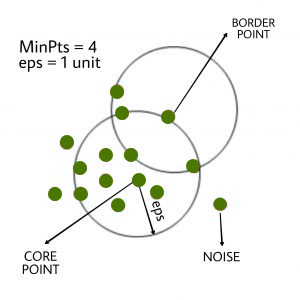
The diagram shows DBSCAN clustering where core points have ≥ 4 neighbors within a 1-unit radius, border points are near core points but not dense enough, and noise points lie outside any dense region.
Implementation of DBScan Clustering in R
We implement the DBScan clustering algorithm in R to identify non-linear clusters and detect noise in an unsupervised learning setting.
1. Installing and Loading Required Packages
We install and load the fpc package which provides the DBScan functionality.
- install.packages: used to install external packages.
- library: used to load the installed package into the session.
install.packages("fpc")
library(fpc)
2. Loading and Viewing the Dataset
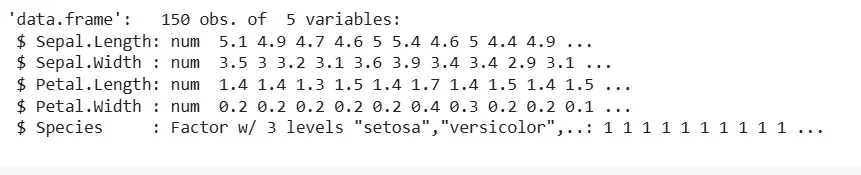
We load and view the built-in Iris dataset to understand its structure.
- data: used to load built-in datasets.
- str: used to view the structure of the dataset.
data(iris)
str(iris)
Output:
3. Preparing the Data for Clustering
We remove the label column to prepare the dataset for unsupervised clustering.
- [-5]: used to exclude the fifth column (Species) from the dataset.
iris_1 <- iris[-5]
4. Fitting the DBScan Model
We fit the DBScan clustering model on the prepared dataset with specified parameters.
- set.seed: used to fix random initialization for reproducibility.
- dbscan: used to apply the DBScan clustering algorithm.
- eps: defines the radius of the neighborhood.
- MinPts: defines the minimum number of points in a neighborhood to form a cluster.
set.seed(220)
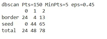
Dbscan_cl <- dbscan(iris_1, eps = 0.45, MinPts = 5)
Dbscan_cl
Output:
5. Checking Cluster Assignments
We extract the cluster assignments and compare them to the original species for evaluation.
- $cluster: used to access the cluster labels.
- table: used to compare actual species with cluster assignments.
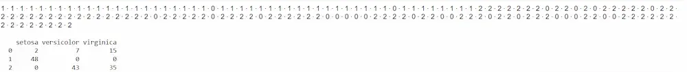
Dbscan_cl$cluster
table(Dbscan_cl$cluster, iris$Species)
Output:
6. Plotting the Clusters
We visualize the clusters to understand the spatial groupings formed by DBScan.
- plot: used to plot the clustered data in 2D space.
plot(Dbscan_cl, iris_1, main = "DBScan")
plot(Dbscan_cl, iris_1, main = "Petal Width vs Sepal Length")
Output:
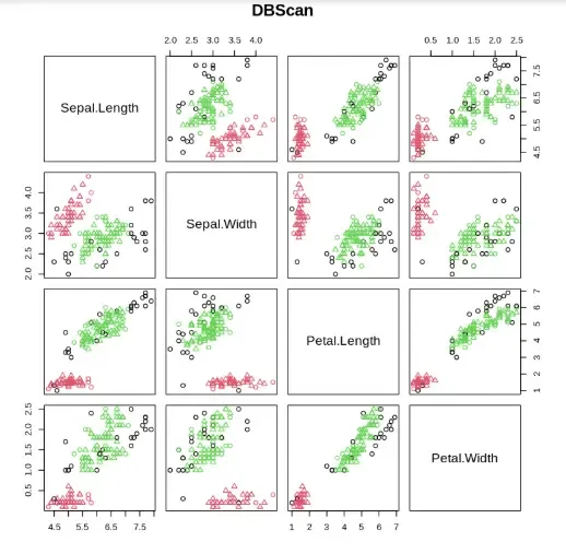
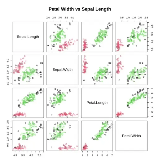
The output displays a 2D scatter plot of DBSCAN clustering results, where points are colored by cluster labels and noise points are marked separately, helping visualize spatial groupings in the Iris dataset.