Data Cleaning in R

Data cleaning is the process of identifying and correcting errors, inconsistencies and inaccuracies in a dataset before analysis. It ensures that the data is reliable, well-structured and ready for meaningful interpretation. Proper data cleaning improves the accuracy of statistical results and machine learning models. It involves:

• Handles missing, incorrect or duplicate values in datasets.
• Standardizes data formats and structures for consistency.
• Prepares raw data for accurate analysis and modeling.

How it Works

Data cleaning in R transforms raw datasets into reliable, analysis-ready information by detecting and correcting issues such as incorrect data types, missing values, formatting inconsistencies and validation errors. This structured workflow ensures data accuracy and consistency before performing statistical analysis or building machine learning models.

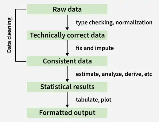
1. Raw Data

This is the original data collected from sources like CSV files, Excel sheets, databases, APIs or surveys. It often contains issues such as:

• Missing or unclear column names
• Incorrect data types
• Duplicate rows
• Missing (NA) values
• Inconsistent formats or extra spaces

At this stage, the data is unclean and not ready for analysis.

2. Technically Correct Data

The dataset is properly imported into R and basic structural fixes are applied.

• Meaningful column names are assigned
• Data types are corrected
• Duplicates are removed
• Missing values are identified

The data is now organized and ready for deeper cleaning.

3. Consistent and Validated Data

The dataset is cleaned, standardized and logically verified.

• Missing values are handled
• Categories and formats are standardized
• Outliers are checked
• Value ranges are validated

At this stage, the data is fully ready for analysis and modeling

Step By Step Implementation

Step 1: Install and Load Required Libraries

Installs and loads the necessary R packages for data manipulation, cleaning, visualization and correlation analysis.

install.packages(c("tidyverse", "skimr", "janitor", "corrplot"))

library(tidyverse)
library(skimr)
library(janitor)
library(corrplot)

Step 2: Load the Dataset and Preview Data

Here we load the built-in airquality dataset and examine its structure and summary statistics.

• head() shows the first 6 rows.
• summary() provides statistical summaries and missing value counts.
• skim() gives a detailed overview including data types and NA values.

air_df <- airquality
head(air_df)
summary(air_df)
skim(air_df)

Output:

Step 3: Check Missing Value Percentage

Here we calculates the percentage of missing values in each column.

sapply(air_df, function(x) sum(is.na(x)) / length(x) * 100)

Output:

Ozone 24.1830065359477 Solar.R 4.57516339869281 Wind 0 Temp 0 Month 0 Day 0

Step 4: Remove Duplicate Rows

This ensures that no duplicate records exist in the dataset.

air_df <- air_df %>% distinct()

Step 5: Clean Column Names

Standardizes column names to lowercase and consistent format.

air_df <- air_df %>% clean_names()
colnames(air_df)

Output:

'ozone' 'solar_r' 'wind' ' temp' 'month' 'day'

Step 6: Handle Missing Values Using Median Imputation

Replaces missing values in ozone and solar_r with their median values.

air_df <- air_df %>%
  mutate(
    ozone = ifelse(is.na(ozone), median(ozone, na.rm = TRUE), ozone),
    solar_r = ifelse(is.na(solar_r), median(solar_r, na.rm = TRUE), solar_r)
  )

Step 7: Correct Data Types and Create Date Column

Convert month into factor and create a proper date column.

air_df$month <- as.factor(air_df$month)
air_df$date <- as.Date(paste(1973, air_df$month, air_df$day, sep = "-"))

Step 8: Define Outlier Capping Function (IQR Method)

Creates a reusable function to detect and cap outliers using IQR. cap_outliers function limits extreme values within calculated lower and upper bounds.

cap_outliers <- function(x) {
  Q1 <- quantile(x, 0.25, na.rm = TRUE)
  Q3 <- quantile(x, 0.75, na.rm = TRUE)
  IQR_val <- Q3 - Q1
  lower <- Q1 - 1.5 * IQR_val
  upper <- Q3 + 1.5 * IQR_val
  x <- pmin(pmax(x, lower), upper)
  return(x)
}

Step 9: Apply Outlier Treatment

Apply the outlier capping function to numeric columns. Extreme values are capped within acceptable IQR limits.

air_df$ozone   <- cap_outliers(air_df$ozone)
air_df$solar_r <- cap_outliers(air_df$solar_r)
air_df$wind    <- cap_outliers(air_df$wind)
air_df$temp    <- cap_outliers(air_df$temp)

Step 10: Feature Engineering

Create a new categorical variable based on temperature. temp_category classifies temperature as Low, Medium or High.

air_df <- air_df %>%
  mutate(temp_category = case_when(
    temp < 70 ~ "Low",
    temp >= 70 & temp < 85 ~ "Medium",
    TRUE ~ "High"
  ))

Step 11: Visualize Cleaned Data

Visualize the cleaned numeric variables using boxplots to examine data distribution and confirm that extreme outliers have been effectively controlled.

boxplot(air_df[, c("ozone", "solar_r", "wind", "temp")],
        main = "Boxplot After Cleaning")

Output:

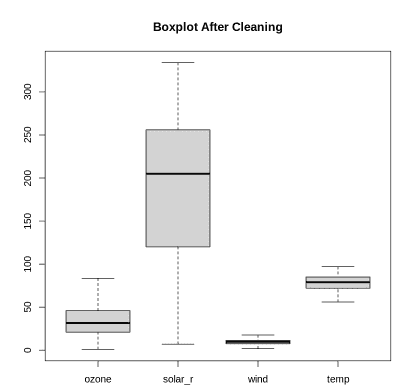
The boxplot shows that after cleaning, there are no extreme outliers, indicating they were properly treated or removed. Solar radiation has the highest variability, while wind has the lowest median and smallest spread.

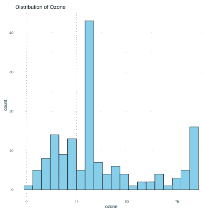
Step 12: Distribution of Ozone

Here we creates a histogram to visualize the distribution of ozone levels in the cleaned dataset. It helps in understanding the frequency pattern and overall spread of ozone values after preprocessing.

ggplot(air_df, aes(x = ozone)) +
  geom_histogram(bins = 20, fill = "skyblue", color = "black") +
  theme_minimal() +
  labs(title = "Distribution of Ozone")

Output:

Step 13: Data Inspection and Verification

Here we reviews the cleaned dataset to confirm that all transformations and preprocessing tasks have been applied correctly.

head(air_df)
summary(air_df)

Output:

Download full code from here.