Transfer learning is a technique where a model trained on one task is reused for a related task, especially when the new task has limited data. This helps in the following ways:
- Uses learned features from the first task
- Reduces training time for the new task
- Improves accuracy with less data
- Uses general features that work across tasks
Importance of Transfer Learning
- Limited Data: Acquiring extensive labelled data is often challenging and costly. Transfer learning enables us to use pre-trained models, reducing the dependency on large datasets.
- Enhanced Performance: Starting with a pre-trained model which has already learned from substantial data allows for faster and more accurate results on new tasks ideal for applications needing high accuracy and efficiency.
- Time and Cost Efficiency: Transfer learning shortens training time and conserves resources by utilizing existing models hence eliminating the need for training from scratch.
- Adaptability: Models trained on one task can be fine-tuned for related tasks making transfer learning versatile for various applications from image recognition to natural language processing.
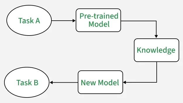
Working of Transfer Learning
- Pre-trained Model: Start with a model already trained on a large dataset for a specific task. This pre-trained model has learned general features and patterns that are relevant across related tasks.
- Base Model: This pre-trained model, known as the base model, includes layers that have processed data to learn hierarchical representations, capturing low-level to complex features.
- Transfer Layers: Identify layers within the base model that hold generic information applicable to both the original and new tasks. Lower layers capture general features such as edges and textures, while higher layers capture task-specific complex patterns.
- Fine-tuning: Fine-tune these selected layers with data from the new task. This process helps retain the pre-trained knowledge while adjusting parameters to meet the specific requirements of the new task, improving accuracy and adaptability.
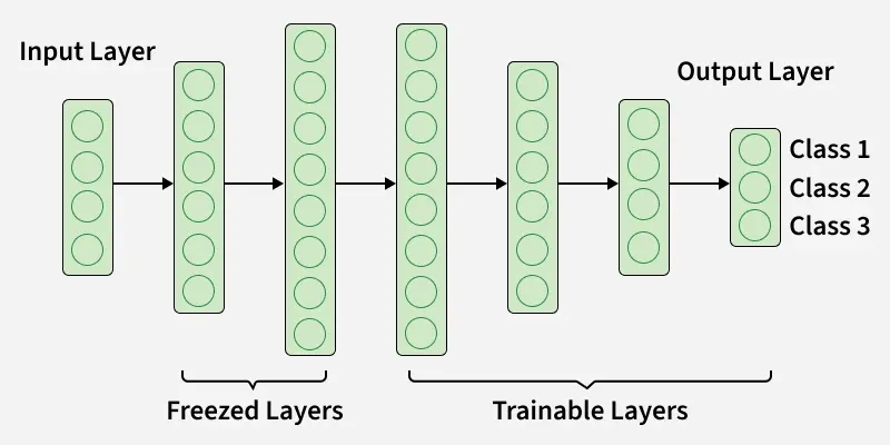
Frozen vs. Trainable Layers in Transfer Learning
| Aspect | Frozen Layers | Trainable Layers |
|---|---|---|
| Definition | Layers whose weights are kept fixed and not updated during training | Layers whose weights are updated during training |
| Purpose | Preserve general features learned from large pre-trained datasets | Adapt to task-specific features of the new dataset |
| Learning Process | No backpropagation updates; remain constant | Updated through backpropagation based on new data |
| Use Case | Used when new dataset is small or similar to the original dataset | Used when new dataset is large or significantly different from the original task |
| Computation Cost | Lower, since fewer parameters are trained | Higher, as more parameters need to be updated |
| Example in CNN | Early convolutional layers that capture edges, textures and basic shapes | Later fully connected layers or deeper convolutional layers for fine-tuned features |
How to Decide Which Layers to Freeze or Train
The extent to which you freeze or fine-tune layers depends on the similarity and size of your target dataset:
- Small, Similar Dataset: For smaller datasets that resemble the original dataset, you freeze most layers and only fine-tune the last one or two layers to prevent overfitting.
- Large, Similar Dataset: With large, similar datasets you can unfreeze more layers allowing the model to adapt while retaining learned features from the base model.
- Small, Different Dataset: For smaller, dissimilar datasets, fine-tuning layers closer to the input layer helps the model learn task-specific features from scratch.
- Large, Different Dataset: In this case, fine-tuning the entire model helps the model adapt to the new task while using the broad knowledge from the pre-trained model.
Transfer Learning with MobileNetV2 for MNIST Classification
In this section, we’ll explore transfer learning by fine-tuning a MobileNetV2 model pre-trained on ImageNet for classifying MNIST digits.
1. Preparing the Dataset
We start by loading the MNIST dataset. Since MobileNetV2 is pre-trained on three-channel RGB images of size 224 x 224, we make a few adjustments to match its expected input shape:
- Reshape the images from grayscale (28 x 28, 1 channel) to RGB (28 x 28, 3 channels).
- Resize images to 32 x 32 pixels, aligning with our model’s configuration.
- Normalize pixel values to fall between 0 and 1 by dividing by 255.
from tensorflow.keras.datasets import mnist
import numpy as np
from tensorflow.keras.utils import to_categorical

(train_images, train_labels), (test_images, test_labels) = mnist.load_data()

train_images = np.stack([train_images]*3, axis=-1) / 255.0
test_images = np.stack([test_images]*3, axis=-1) / 255.0

train_images = tf.image.resize(tf.convert_to_tensor(train_images), [32, 32])
test_images = tf.image.resize(tf.convert_to_tensor(test_images), [32, 32])

train_labels = to_categorical(train_labels, 10)
test_labels = to_categorical(test_labels, 10)
2. Building the Model
We load MobileNetV2 with pre-trained weights from ImageNet excluding the fully connected top layers to customize for our 10-class classification task:
- Freeze the base model to retain learned features and avoid overfitting.
- Add a global average pooling layer to reduce model complexity.
- Add a dense layer with softmax activation for the output classes.
from tensorflow.keras.applications import MobileNetV2
from tensorflow.keras.layers import Input, GlobalAveragePooling2D, Dense
from tensorflow.keras.models import Model

base_model = MobileNetV2(weights='imagenet', include_top=False, input_shape=(32, 32, 3))
base_model.trainable = False  # Freeze base model

inputs = Input(shape=(32, 32, 3))
x = base_model(inputs, training=False)
x = GlobalAveragePooling2D()(x)
outputs = Dense(10, activation='softmax')(x)
model = Model(inputs, outputs)
Output:
base_model=MobileNetV2(weights='imagenet', include_top=False, input_shape=(32, 32, 3))
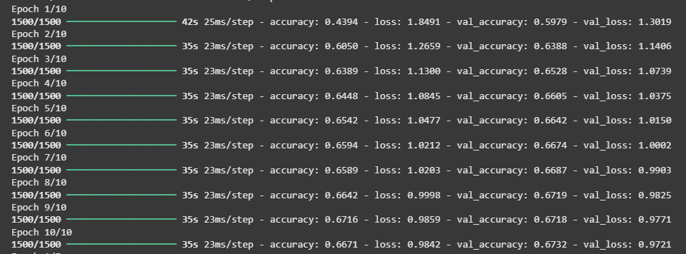
3. Compiling and Training the Model
The model is compiled with categorical cross-entropy as the loss function and accuracy as the evaluation metric. Using Adam optimizer we train the model on the MNIST training data for ten epochs.
model.compile(optimizer='adam', loss='categorical_crossentropy', metrics=['accuracy'])
model.fit(train_images, train_labels, epochs=10, validation_split=0.2)
Output:
4. Fine-Tuning the Model
After initial training we unfreeze the last few layers of the base model to perform fine-tuning. This allows the model to adjust high-level features for the MNIST data while retaining its foundational knowledge.
base_model.trainable = True
for layer in base_model.layers[:100]:
    layer.trainable = False

model.compile(optimizer=tf.keras.optimizers.Adam(1e-5), loss='categorical_crossentropy', metrics=['accuracy'])
model.fit(train_images, train_labels, epochs=5, validation_split=0.2)
Output:
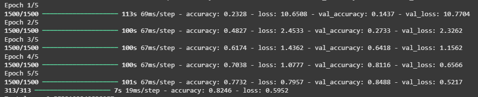
5. Model Evaluation
Once the model has been trained and fine-tuned we evaluate it on the test set, measuring its loss and accuracy. This step assesses how well the transfer learning model has adapted to the MNIST dataset and demonstrates its effectiveness in digit classification.
loss, accuracy = model.evaluate(test_images, test_labels)
print(f"Test loss: {loss}")
print(f"Test accuracy: {accuracy}")
Output:
Test loss: 0.5697252154350281
Test accuracy: 0.8434000015258789
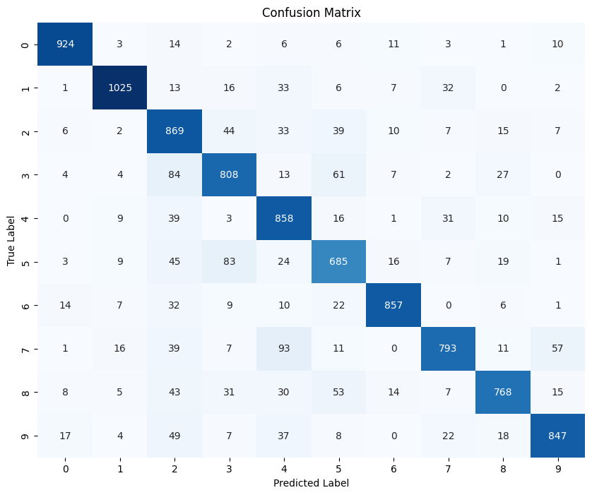
6. Visualizing Model Performance
To visualize the performance further a confusion matrix provides a breakdown of correct and incorrect classifications.
from sklearn.metrics import confusion_matrix
import seaborn as sns
import matplotlib.pyplot as plt

test_predictions = model.predict(test_images)
test_predictions_classes = np.argmax(test_predictions, axis=1)
test_true_classes = np.argmax(test_labels, axis=1)

cm = confusion_matrix(test_true_classes, test_predictions_classes)
plt.figure(figsize=(10, 8))
sns.heatmap(cm, annot=True, fmt='d', cmap='Blues', cbar=False)
plt.xlabel('Predicted Label')
plt.ylabel('True Label')
plt.title('Confusion Matrix')
plt.show()
Output:
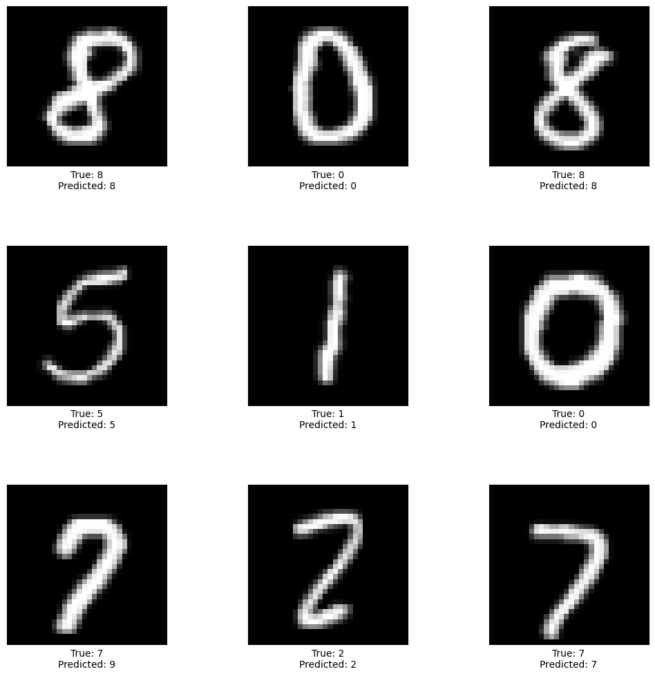
7. Sample Image Visualization
Finally we select a few test images to visualize the model’s predictions against their true labels.
def display_sample(sample_images, sample_labels, sample_predictions):
    fig, axes = plt.subplots(3, 3, figsize=(12, 12))
    fig.subplots_adjust(hspace=0.5, wspace=0.5)

    for i, ax in enumerate(axes.flat):
        ax.imshow(sample_images[i].reshape(32, 32), cmap='gray')
        ax.set_xlabel(f"True: {sample_labels[i]}\nPredicted: {sample_predictions[i]}")
        ax.set_xticks([])
        ax.set_yticks([])

    plt.show()

test_images_gray = np.dot(test_images[...,:3], [0.2989, 0.5870, 0.1140])

random_indices = np.random.choice(len(test_images_gray), 9, replace=False)
sample_images = test_images_gray[random_indices]
sample_labels = test_true_classes[random_indices]
sample_predictions = test_predictions_classes[random_indices]
display_sample(sample_images, sample_labels, sample_predictions)
Output:
Download the source code from here.
Applications
- Computer Vision: Used in image recognition where pre-trained models are adapted for tasks like medical imaging, facial recognition and object detection.
- Natural Language Processing (NLP): Models like BERT, GPT and ELMo are pre-trained on large text data and fine-tuned for tasks such as sentiment analysis and question answering.
- Healthcare: Helps in building diagnostic systems by applying learned features to medical images like X-rays and MRIs.
- Finance: Used for fraud detection, risk assessment and credit scoring by transferring patterns from related financial data.
Advantages
- Speed up the training process: Speeds up training by using a pre-trained model that already understands important features and patterns.
- Better performance: Improves performance on the new task by leveraging knowledge learned from the previous task.
- Handling small datasets: Works well with limited data by using general features, helping to reduce overfitting.
Limitations
- Domain mismatch: The pre-trained model may perform poorly if the source and target tasks or data distributions are very different.
- Overfitting: Excessive fine-tuning can make the model too task-specific, reducing generalization.
- Complexity: Requires high computational resources and may need specialized hardware.