Introduction To Adam Optimizer

Adam (Adaptive Moment Estimation) optimizer combines the advantages of Momentum and RMSprop techniques to adjust learning rates during training. It works well with large datasets and complex models because it uses memory efficiently and adapts the learning rate for each parameter automatically.

Working of Adam Optimizer

Adam combines two optimization techniques, Momentum and RMSProp, to achieve faster and more stable training.

1. Momentum

Momentum accelerates gradient descent by using a moving average of past gradients, helping reduce oscillations and speed up convergence. The update rule with momentum is:

w_{t+1} = w_{t} - \alpha m_{t}

where:

• m_t is the moving average of the gradients at time t
• α is the learning rate
• w_t​ and w_{t+1}​ are the weights at time t and t+1, respectively

The momentum term m_t is updated recursively as:

m_{t} = \beta_1 m_{t-1} + (1 - \beta_1) \frac{\partial L}{\partial w_t}

where:

• \beta_1​ is the momentum parameter (typically set to 0.9)
• \frac{\partial L}{\partial w_t}​ is the gradient of the loss function with respect to the weights at time t

2. RMSprop (Root Mean Square Propagation)

RMSprop is an adaptive learning rate optimization method that improves AdaGrad by using an exponentially weighted moving average of squared gradients. This prevents the learning rate from decreasing too quickly during training. The update rule for RMSprop is:

w_{t+1} = w_{t} - \frac{\alpha_t}{\sqrt{v_t + \epsilon}} \frac{\partial L}{\partial w_t}

where:

• v_t​ is the exponentially weighted average of squared gradients:

v_t = \beta_2 v_{t-1} + (1 - \beta_2) \left( \frac{\partial L}{\partial w_t} \right)^2

• ϵ is a small constant (e.g., 10^{-8}) added to prevent division by zero

Combining Momentum and RMSprop to form Adam Optimizer

Adam optimizer combines the momentum and RMSprop techniques to provide a more balanced and efficient optimization process. The key equations governing Adam are as follows:

• First moment (mean) estimate:

m_t = \beta_1 m_{t-1} + (1 - \beta_1) \frac{\partial L}{\partial w_t}

• Second moment (variance) estimate:

v_t = \beta_2 v_{t-1} + (1 - \beta_2) \left( \frac{\partial L}{\partial w_t} \right)^2

• Bias correction: Since both m_t​ and v_t are initialized at zero, they tend to be biased toward zero, especially during the initial steps. To correct this bias, Adam computes the bias-corrected estimates:

\hat{m_t} = \frac{m_t}{1 - \beta_1^t}, \quad \hat{v_t} = \frac{v_t}{1 - \beta_2^t}

• Final weight update: The weights are then updated as:

w_{t+1} = w_t - \frac{\hat{m_t}}{\sqrt{\hat{v_t}} + \epsilon} \alpha

Key Parameters

• α: The learning rate or step size (default is 0.001)
• \beta_1​ and \beta_2​: Decay rates for the moving averages of the gradient and squared gradient, typically set to \beta_1 = 0.9 and \beta_2 = 0.999
• ϵ: A small positive constant (e.g., 10^{-8}) used to avoid division by zero when computing the final update

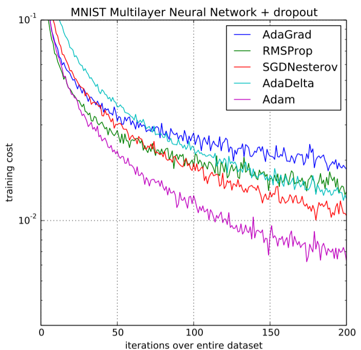
Performance of Adam Optimizer

Adam delivers strong performance in training deep learning models and large datasets by combining adaptive learning rates with momentum.

• Uses adaptive learning rates for each parameter based on past gradients and their magnitudes
• Helps reduce oscillations and move past local minima effectively
• Applies bias correction to prevent instability during early training stages
• Requires less hyperparameter tuning compared to optimizers like SGD
• Provides efficient, stable, and reliable optimization across different tasks

Implementation

Step 1: Install Required Libraries

• TensorFlow/Keras is used for building and training neural networks
• NumPy handles numerical computations and arrays
• Matplotlib is used for visualization and plotting
• Scikit-learn provides dataset utilities and preprocessing tools
• Run the following command in your terminal

pip install tensorflow numpy matplotlib scikit-learn

Step 2: Import Required Libraries

• make_moons() generates a non-linear classification dataset
• train_test_split() divides data into training and testing sets
• StandardScaler() normalizes the data
• Sequential() creates a neural network model
• Dense() adds fully connected layers
• Adam() applies the Adam optimizer

import numpy as np
import matplotlib.pyplot as plt

from sklearn.datasets import make_moons
from sklearn.model_selection import train_test_split
from sklearn.preprocessing import StandardScaler

from tensorflow.keras.models import Sequential
from tensorflow.keras.layers import Dense
from tensorflow.keras.optimizers import Adam

Step 3: Create Dataset

Generate a synthetic dataset for binary classification.

• n_samples=1000 creates 1000 data points
• noise=0.2 adds slight randomness for realistic data
• random_state=42 ensures reproducibility

X, y = make_moons(n_samples=1000, noise=0.2, random_state=42)

Step 4: Split the Dataset

Divide the dataset into training and testing sets.

• 80% of data is used for training
• 20% of data is reserved for testing
• Helps evaluate model generalization

X_train, X_test, y_train, y_test = train_test_split(
    X, y, test_size=0.2, random_state=42
)

Step 5: Normalize the Data

Feature scaling improves optimization performance and convergence speed.

• Standardization transforms features to zero mean and unit variance
• Prevents features with large values from dominating training
• Helps Adam optimizer converge faster and more stably

scaler = StandardScaler()

X_train = scaler.fit_transform(X_train)
X_test = scaler.transform(X_test)

Step 6: Build the Neural Network

Create a neural network using fully connected layers.

• First hidden layer contains 16 neurons with ReLU activation
• Second hidden layer contains 8 neurons
• Output layer uses sigmoid activation for binary classification

model = Sequential([
    Dense(16, activation='relu', input_shape=(2,)),
    Dense(8, activation='relu'),
    Dense(1, activation='sigmoid')
])

Step 7: Compile the Model with Adam Optimizer

• Initialize the Adam optimizer with a learning rate.
• Compile the neural network with loss function and evaluation metric.

adam_optimizer = Adam(learning_rate=0.001)
model.compile(
    optimizer=adam_optimizer,
    loss='binary_crossentropy',
    metrics=['accuracy']
)

Step 8: Train the Model

Train the neural network using the training dataset.

• epochs=50 means the dataset is processed 50 times
• batch_size=32 updates weights after every 32 samples
• validation_split=0.2 reserves 20% of training data for validation
• Training history stores loss and accuracy values

history = model.fit(
    X_train,
    y_train,
    epochs=50,
    batch_size=32,
    validation_split=0.2,
    verbose=1
)

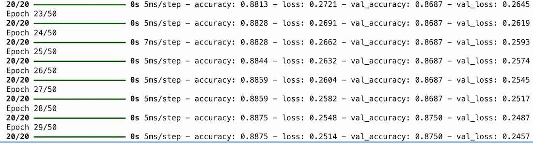
Output:

Step 9: Evaluate the Model

Evaluate model performance on unseen test data.

• Evaluates how well the model generalizes to new data
• Lower loss and higher accuracy indicate better performance

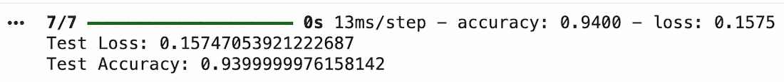
loss, accuracy = model.evaluate(X_test, y_test)

print("Test Loss:", loss)
print("Test Accuracy:", accuracy)

Output:

Download full code from here

Advantages

• Uses adaptive learning rates for each parameter based on past gradients
• Helps reduce oscillations and escape local minima effectively
• Applies bias correction to improve stability during early training stages
• Requires less hyperparameter tuning compared to optimizers like SGD
• Provides efficient optimization across different machine learning tasks

Limitations

• Can sometimes converge to suboptimal solutions compared to SGD
• Requires more memory because it stores additional moment estimates
• Performance is sensitive to hyperparameter selection in some cases
• May generalize less effectively on certain datasets and deep learning tasks
• Can struggle with sparse gradients or very noisy optimization landscapes