Table Visualization in Excel Power View is used to display data in a structured format using rows and columns. It helps users organize, analyze, and explore data easily by selecting relevant fields. This default visualization can also be converted into charts, matrices, cards, or maps for better data insights.
Note: Power View is deprecated in modern Excel versions and may not be available in Excel 2016 and later. Microsoft recommends using Power BI for advanced data visualization.
Switch Table Visualization
Step 1: Click on the Table Visualization
Click on the Table visualization. Two tabs, POWER VIEW, and DESIGN appear on the Ribbon.
Step 2: Click the Design Tab.
You can choose any of the options present in the Switch Visualization group on the Ribbon.
- Matrix Visualizations
- Card Visualizations
- Chart Visualizations
- Map Visualization
Creating Table Visualization
Follow these steps to create a table in Power View:
Step 1: Do the steps to build a Table in Power View: Select the Power View region. In the Power View Fields list, click on the table - Range. Choose from the options of Country, Events, Seasons, and Year.
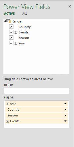
Step 2: As you can see, a Table with selected fields as columns and actual data values will be displayed.

Adding a Table as Count Field
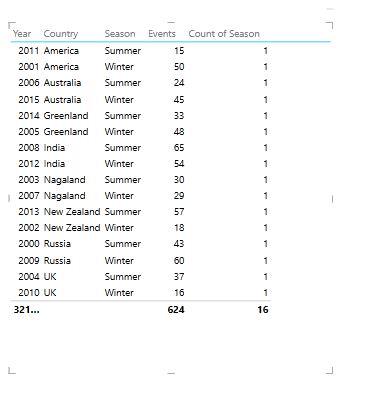
Assume you wish to show the Season Count as a column. You may achieve this by adding the Season field to the Table as Count. In the Power View Fields list, click the arrow next to the Season field. From the dropdown list, choose to Add to Table as Count.
The Table will receive a new column Count of Season, which will display the Season Count values.
Adding a Count Field to Table
When working with large datasets (more than 10,000 rows), adding a Count field directly in Power View can slow down performance because the calculation is repeated each time the layout changes. Instead, creating a calculated field in the Data Model is more efficient.
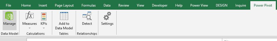
Step 1: On the Ribbon, select the PowerPivot tab. In the Data Model group, choose Manage. The Data Model's tables will be presented.
Step 2: Select the Results tab. In the Results table, in the calculation area, in the cell below the Season column, enter the DAX (Data Analysis Expressions) formula shown below:
Season Count: =COUNTA([Season])
The Season count formula is shown in the formula bar. When you hover over a Season value, then it will show the Season Count i.e.,16 in this case.

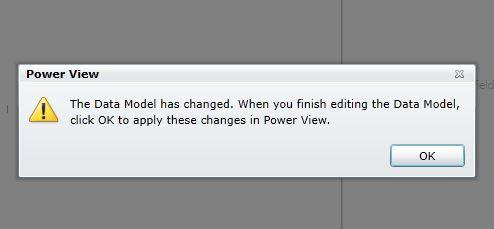
Step 3: Again, you will get a Power View notification indicating that the Data Model has been altered, and if you click OK, the changes will be reflected in your Power View. Select OK.
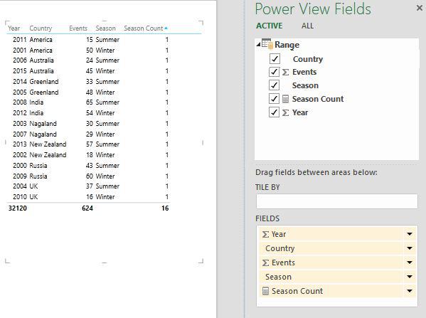
Step 4: Select Country, Events, Season, Season Count, and Year to display the season-wise count in the table.
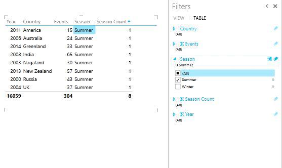
Filtering Table in Power View
In the Filters pane, select the TABLE tab. Choose the Season field and switch to Advanced Filter mode.
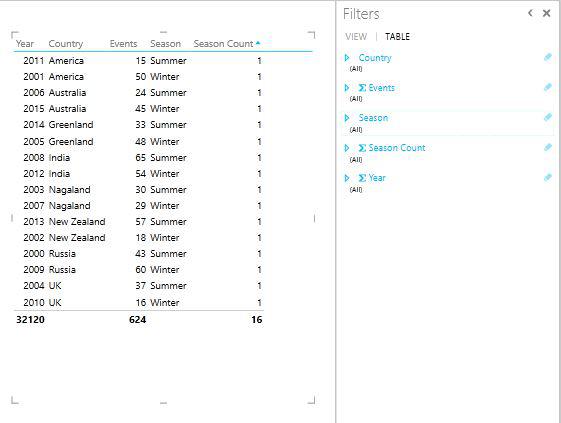
Select Summer and click Apply Filter. The table will now display only records related to the Summer season.