A survival curve is a chart that shows the probability of individuals surviving over time. It helps track how many people remain alive or free from a specific event during a study. In Microsoft Excel, a survival curve can be created by organizing survival data and plotting it using charts like a scatter plot.
Creating a Survival Curve in Excel
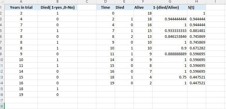
Assume we have the accompanying dataset that shows how long a patient was in a clinical preliminary (section A) and regardless of whether or not the patient was as yet alive toward the finish of the preliminary (segment B).

To make an endurance bend for this information, we want to initially get the information in the right configuration, then utilize the implicit Excel diagrams to make the bend.
Formatting the Data
Utilize the accompanying moves toward getting the information in the right organization.
Step 1: List all of the special "Years in trial" values in column A in column D:
Note: Always incorporate "0" as the primary worth.

Step 2: Make the qualities in segments E through H utilizing the recipes displayed beneath. Here are the equations utilized in the accompanying cells:
E3=COUNTIFS($A$2:$A$16,D3,$B$2:$B$16,1)
F2=COUNTIF($A$2:$A$16, “>”&D2-1)
G3: =1-(E3/F3)
H2: =1
H3: =H2*G3
To fill in every one of the different qualities in section E, basically feature the reach E4:E13 and press Ctrl-D. Fill in each of the different qualities in segments F through H utilizing a similar stunt.
Presently we're prepared to make the endurance bend.
Creating the Survival Curve
Utilize the accompanying moves to make the endurance bend.
Step 1: Duplicate the qualities in sections D and H into segments J and K.
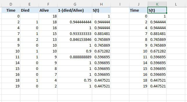
Step 2: Duplicate the qualities in the reach J3:J14 to J15:J26. Then duplicate the qualities in the reach K2:K13 to K15:K26.
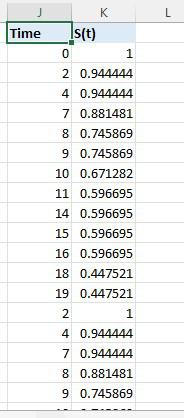
Step 3: Make a rundown of values in segment L as displayed underneath, then, at that point, sort from littlest to biggest qualities in section L:
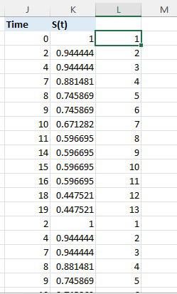
Step 4: Sort columns J through L smallest to largest based on column L

Step 5: Highlight cells J2:K26, then select “Insert” > “Charts|Scatter” > “Scatter with Straight Lines and Markers” option.
