Creating a chart from multiple sheets in Excel allows you to consolidate and visualize data from different worksheets in a single, cohesive chart. This technique is useful for comparing datasets across tabs, tracking trends, and presenting comprehensive insights without manually combining data.
How to Create a Chart from Multiple Sheets in Excel
Assuming you have a couple of worksheets with income information for various years and you need to make an outline in light of that information to picture the general pattern.
Step 1: Select Data for the Graph
Open your first Excel worksheet and select the data you need to plot in the graph. Highlight the relevant information to ensure it is included in the chart.

Step 2: Choose a Chart Type
Go to the Insert tab and, in the Charts group, select the type of graph you need to create. Choose the appropriate chart style based on your data and desired presentation.

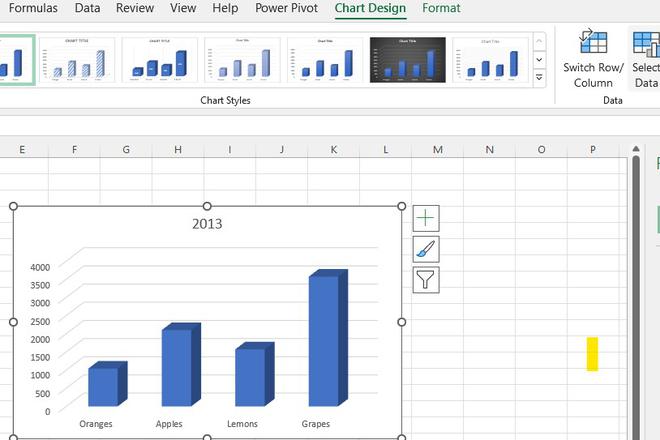
Step 3: Select the Stacked Column Chart
In this model, we will create a Stacked Column chart. Select the Stacked Column option from the chart types available to visualize your data effectively.

Step 4: View the Result
Below is the result of the stacked column chart created from your selected data, visually representing the values in a clear and organized manner.

How to a Second Data Series from Another Sheet
Here are the steps to add a second data series from another sheet in Excel:
Step 1: Activate the Chart Tools
Click on the diagram you've recently created to activate the Chart Tools tabs on the Excel ribbon. This will allow you to make further customizations to your chart.
Step 2: Add a New Data Series
In the Select Data Source window, click the Add button to add a new data series to your chart. This allows you to include additional data from another sheet or source.

Presently we will add the second information series in light of the information situated on an alternate worksheet. This is the central issue, so kindly make certain to adhere to the guidelines intently.
Step 3: Open the Edit Series Window
Clicking the Add button opens the Edit Series window. In this window, click the Collapse Dialog button next to the Series values field to select the data range from another sheet.

Step 4: Select the Data from Another Sheet
The Edit Series window will shrink to allow access to a smaller selection window. Click on the tab of the sheet that contains the additional information you need for your Excel graph. The Edit Series window will remain open as you navigate between sheets.

Step 5: Select Data from the Other Worksheet
On the subsequent worksheet, select the range or line of data you need to add to your Excel chart. After selecting the data, click the Expand Dialog icon to return to the regular Edit Series window.

Step 6: Set the Series Name and Confirm the Data
Next, click the Collapse Dialog button to the left of the Series Name field. Select the cell containing the text you want to use as the series name. Then, click the Expand Dialog button to return to the original Edit Series window. Ensure the references in both the Series Name and Series Values boxes are correct, and then click the OK button to confirm the changes.

Step 7: Add a Series Name
As shown in the screenshot above, the series name is linked to cell B1, which contains a section name. Alternatively, you can type your own series name in double quotes, e.g., ="Second Data Series". These names will appear in the chart legend, so make sure to give meaningful and descriptive names to your data series. The outcome should now look similar to this:

Modify an Excel Chart Built from Multiple Sheets
After creating a chart from two or more sheets, you might want to change how it looks. Editing the existing chart is usually easier than making a new one from scratch.

Also, to change the information series plotted in the graph, there are three methods for doing this:
- Select the Data Source dialog
- Chart Filters button
- Data series formulas