The SUMIF function in Excel adds values from a range that meet a specific condition. It helps you quickly calculate totals based on criteria like text, numbers, or dates, such as summing sales for a category or values within a certain date. This makes data analysis faster and easier.
The simplest form of SUMIF Formula is:
SUMIF(range, criteria, [sum_range])
- range: The range of cells you want to evaluate based on the criteria.
- criteria: The condition that determines which cells to sum.
- sum_range(optional argument): returns the sum of the sum_range or the range according to the given arguments
Note: sum_range (optional): The range of cells to sum if different from the range to evaluate. If sum range not mentioned, it calculates the sum of same range as criteria condition.
Return Value:
This function sums the numbers in the given range and returns the numerical value of the sum.
SUMIF Function in Excel
The SUMIF function is a useful tool, but it only takes a few simple steps to use it effectively. Here are the following steps to effectively use SUMIF in Excel formula.
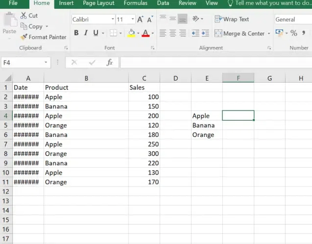
Step 1: Open MS Excel
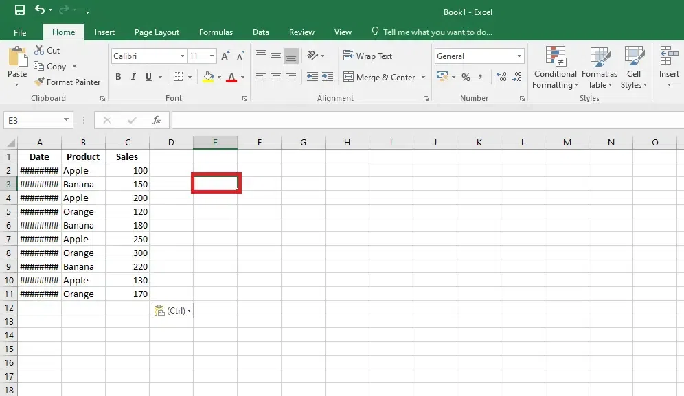
Step 2: Select the Cell for the Result
Select the cell in which you want to display the result of the SUMIF Function.
Step 3: Enter the SUMIF Function and specify the range
Start typing the Formula starting with the '=SUMIF' in the selected cell and also specify the range of the cells you want to evaluate. For example, if you want to evaluate cells 'B2' to 'B11', type 'B2:B11',.
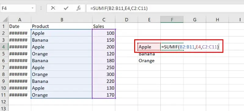
Step 4: Define the Criteria
Enter the criteria for summing the values. For example, if you want to sum cells where the value is "Apple", Select cell E4(Apple).
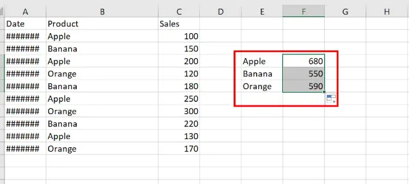
Step 5: Drag the Formula
Step 6: Preview the Result
Excel SUMIF with Dates
The SUMIF function with dates allows you to add values based on specific date criteria, ideal for tracking sales or events within a certain timeframe. For example, to sum all values after January 1, 2023, enter =SUMIF(B2:B11, ">01/01/2023", C2:C11).
Step 1: Open MS Excel
Step 2: Select the Cell
Select the cell in which you want to display the output.
Step 3: Enter the SUMIF Function and specify the range
Start by typing =SUMIF( in the selected cell and enter the range of cells the dates you want to evaluate. For example, if your dates are in column B from B2to B10, type B2:B10,.

Step 4: Define the Criteria
Enter the date criteria. For instance, if you want to sum values for dates after January 1, 2023, type " >01/01/2023",.

Step 5: Enter the Sum Range
Enter the range of cells that contain the values you want to sum. For example, if these values are in column B from B2 to B10, type B2:B10).

Example of SUMIF Function
An Excel sheet has been taken as an example and the SUMIF function has been used in several formats.
Input:
| Coding Team names(Column A) | No. of members(Column B) | points(Column C) |
|---|---|---|
| GFG_CODERS | 4 | 200 |
| Acex_coders | 5 | 197 |
| Poisionous_python | 3 | 150 |
| Megatron | 4 | 130 |
| Bro_coders | 6 | 110 |
| Kotlin_coders | 2 | 100 |
| Gaming_coders | 3 | 50 |
Then we will apply the SUMIF() function to the above table:
| SUMIF() function | What the function does | Output result |
|---|---|---|
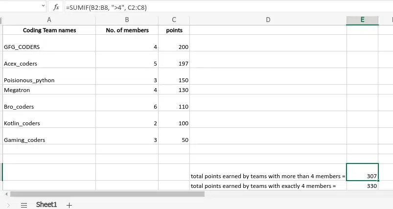
| =SUMIF(B2:B8, ">4", C2:C8) | If the no. of members in column B is greater than 4 then add the corresponding points of column C. | 307 |
| =SUMIF(B2:B8, 4, C2:C8) | If the no. of members in column B is equal to 4 then add the corresponding points of column C. | 330 |
| =SUMIF(A2:A8, "GFG_CODERS", C2:C8) | Search for "GFG_CODERS" in column A and add the corresponding points in column C. | 200 |
| =SUMIF(C2:C8, ">110") | Here the sum_range argument is not provided. So it will check the cells of C column and if the points are greater than 110 add it to the result. | 677 |
| =SUMIF(A2:A8, "*rs", C2:C8) | Here it will find the names of the teams ending with "rs" / "RS" in column A and add the corresponding points to the sum. | 657 |
Output:
SUMIFS with Multiple Criteria in Spreadsheet
Below are some examples of SUMIF Function in Excel:
Step 1: Enter the data Set
Step 2: Enter the Formula for multiple criteria
=SUMIFS(sum_range, criteria_range1, criteria1, [criteria_range2, criteria2], ...)
- sum_range: The range to add.
- criteria_range1, criteria1: The first range and condition pair.
- [criteria_range2, criteria2] (optional): Additional ranges and conditions.
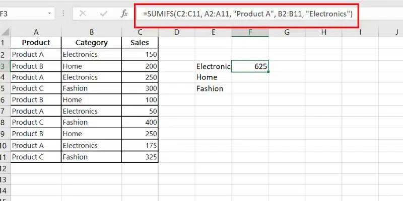
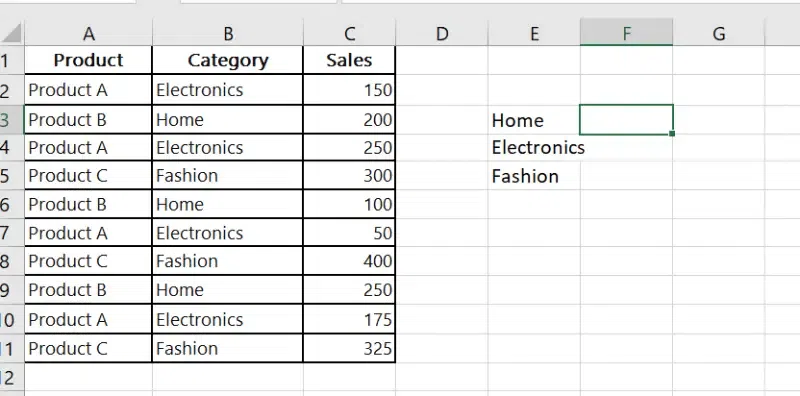
Example: To sum the Sales where Product is "Product A" and Category is "Electronics":
=SUMIFS(C2:C10, A2:A10, "Product A", B2:B10, "Electronics")