The CHOOSE function selects a value from a list based on a number. It simplifies conditional results, replacing complex IFs, and works dynamically with functions like RANDBETWEEN, VLOOKUP, or MONTH.
Excel CHOOSE Function Syntax
Based on a defined location, Excel's CHOOSE function is intended to return a value from the list.
=CHOOSE(index_num, value1, [value2], ...)Parameter
- Index_num: The value we want to choose. The number must be between 1 and 254.
- Value1: The first value from which to choose.
- Value2 (Optional): The second value from which to choose.
Key Features of CHOOSE Function
- Allows selection from up to 254 values.
- Returns #VALUE! if the index is <1 or > number of values.
- If the index is a fraction, the lowest integer is used..
Steps to Use CHOOSE Function in Excel
Let's consider the following examples.
Example 1
To get our Value, follow the below steps
Step 1: Format your Data
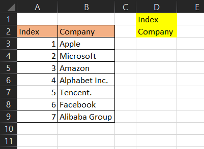
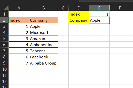
Now, if we want to get the value of any number (index) in E1. Let us follow the next step
Step 2: Enter the Formula
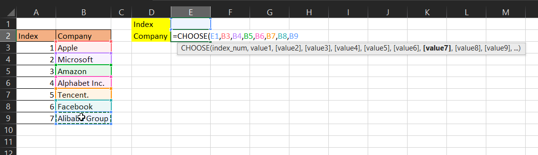
We will enter " =CHOOSE(E1,B3,B4,B5,B6,B7,B8,B9) " in E2 cell.
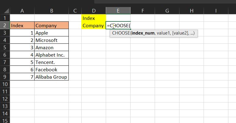
Here we said Excel should return our index (E1) from our list; B3,B4,B5,B6,B7,B8,B9.
This will return a #VALUE! Error because there is no number provided in E1.
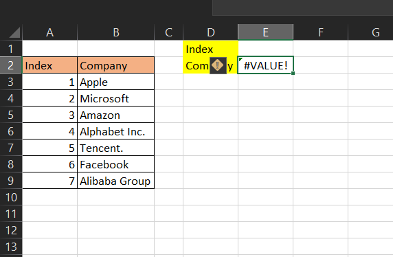
Let's put 1 in E1. The CHOOSE function returns Apple because Apple is the value with index 1 on your list.
Example 2
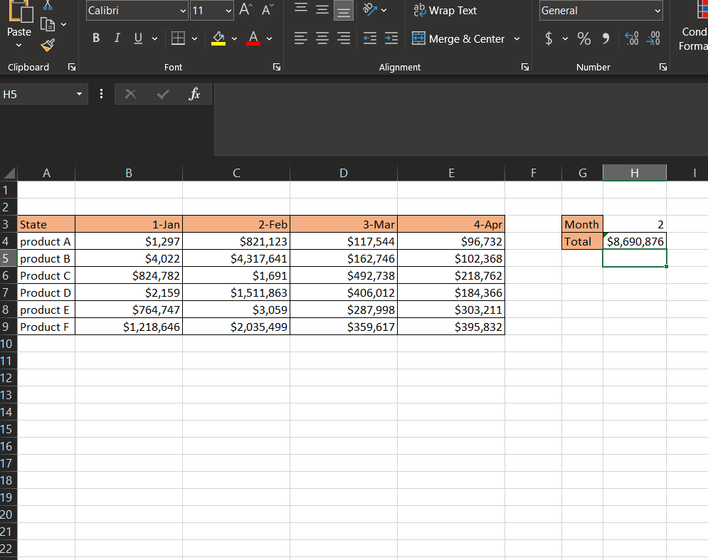
Here we want to pick a month, and we want it to display the sum of revenue for that month picked.
Step 1: Format your Data
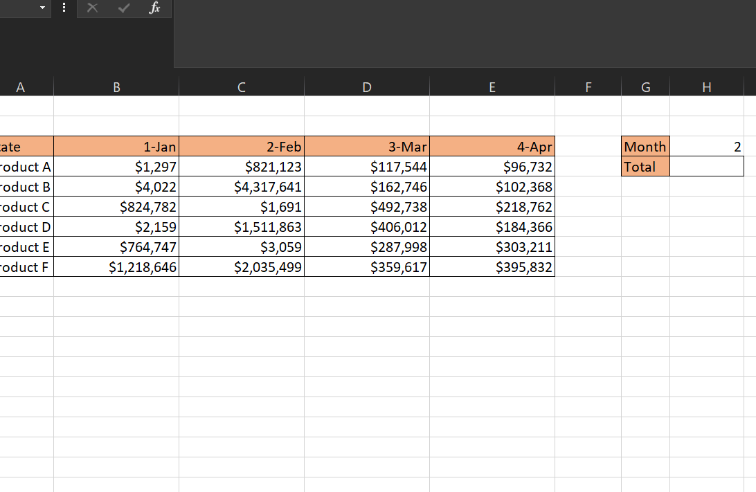
Now, if we want to get the sum of the month picked in H4. Let us follow the next step
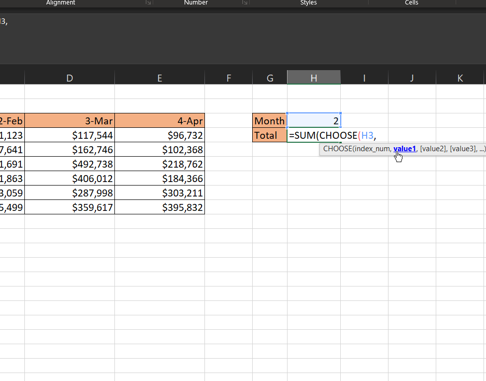
Step 2: Enter SUM(CHOOSE(H3))
In H3, we would put a number 1, 2, or 3 which represents Jan, Feb, and March. Thus, We will enter " =SUM(CHOOSE(H3)) "
Step 3: Enter "=SUM(CHOOSE(H3,B4:B9,C4:C9,D4:D9,E4:E9))"
This will be followed by the values in each month. Thus, This will be We will enter " =SUM(CHOOSE(H3,B4:B9,C4:C9,D4:D9,E4:E9)) " in H4 cell.
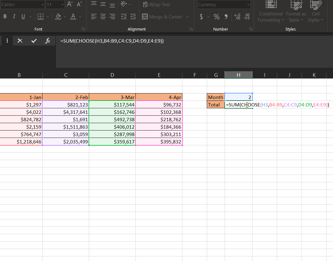
Step 4: Press Enter
Then we press ENTER on our keyboard. This will return the sum of values for 1 which is Jan.
CHOOSE Function in Excel: Purpose and Practical Examples
CHOOSE can simplify tasks like returning different values based on a condition. Instead of using complex nested IFs, CHOOSE offers a quick and easy alternative.
1. Return Different Values Based on the Condition
Supposing you have a column of Air Quality Index and you want to label the scores based on the following conditions:
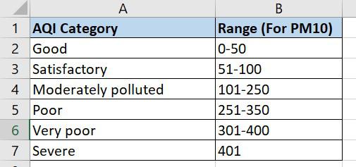
- Nesting a few IF formulae inside of one another is one method for achieving this
=IF(E2>=401, "Severe", IF(E2>=301, "Very poor", IF(E2>=251, "Poor", IF(E2>=101,"Moderately Polluted", IF(E2>=51,"Satisfactory", "Good")))))- Another option is to select a label that fits the condition
=CHOOSE((E2>0) + (E2>=51) + (E2>=101) + (E2>=251) + (E2>=351) + (E2>=401), "Good", "Satisfactory", "Moderately Polluted", "Poor", "Very Poor", "Severe")
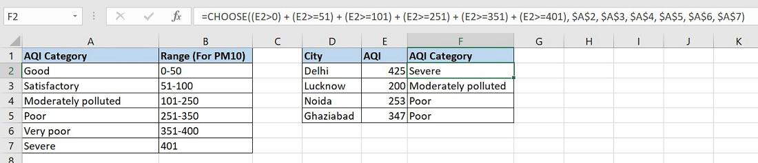
Instead of using hardcoded labels, you can use cell references to increase the formula's flexibility, for example:
=CHOOSE((E2>0) + (E2>=51) + (E2>=101) + (E2>=251) + (E2>=351) + (E2>=401), $A$2, $A$3, $A$4, $A$5, $A$6, $A$7)
2. Excel CHOOSE Formula for Random Data
As you are surely aware, Microsoft Excel includes a unique function called RANDBETWEEN that creates random integers between the bottom and top numbers that you select. It should be nested inside the index num argument of CHOOSE so that your formula can produce practically any kind of random data.
Example:
=CHOOSE(RANDBETWEEN(1,6), "Good", "Satisfactory", "Moderately polluted", "Poor", "Very poor", "Severe")
3. CHOOSE Function for Selecting Month
The CHOOSE function acts like a selector that picks a month from a list based on a given date. For example, if you have a date in Excel and want to determine the corresponding month, you can use the CHOOSE function to retrieve it.
Let's consider you have a list of dates in Column A, and you want to find the month for one of those dates, like the second date in cell A3.
.png)
You can use this formula: "=CHOOSE(MONTH(A4), "Jan", "Feb", "Mar", "Apr", "May","Jun", "Jul", "Aug", "Sep", "Oct", "Nov", "Dec")."
When you use this formula, it checks the month of the date in cell A4 and then gives you the corresponding months name. So, if A4 contains a date in March it will return "Mar".
.png)
Excel CHOOSE Function With VLOOKUP
Utilizing the CHOOSE Function in conjuction with VLOOKUP Function allows for the retrieval off specific desired values. You can refer to the link to learn about " CHOOSE Function With VLOOKUP".
Error in Using CHOOSE Function
It returns "#VALUE! Error" occurs:
- The "noindex_num" argument argument surpasses the available choices.
- The "noindex_num" argument doesn't align with a numeric value.
A "#NAME? Error" emerges when:
- The value arguments are presented as text arguments without enclosing quotes.
- Valid cell references are not furnished as arguments.