Gated Recurrent Units (GRUs) are an advanced type of recurrent neural network designed to efficiently model sequential and time-series data. By using gating mechanisms, GRUs address the vanishing gradient problem common in traditional RNNs, enabling them to capture long-term dependencies with fewer parameters and faster training compared to LSTMs.
- GRUs combine multiple gates into update and reset gates, reducing complexity while retaining the ability to learn long-term patterns.
- Ideal for handling sequences in natural language processing, speech recognition and time-series forecasting.
- Fewer parameters than LSTMs make GRUs faster to train and easier to deploy in resource-constrained environments.
Problems with LSTM
Although LSTM are effective at learning long-term dependencies, they have some limitations that can make them less practical in certain scenarios.
- Complex architecture: LSTMs use multiple gates (input, forget, output), making the network heavier and harder to train.
- More parameters: The large number of parameters increases memory usage and computational cost.
- Slower training: Due to the complex structure, LSTMs often require more time to converge.
- Risk of overfitting: With many parameters, LSTMs can overfit smaller datasets.
- Difficult deployment: Larger models are harder to deploy in resource-constrained environments like mobile devices.
GRU as an Efficient Alternative to LSTM for Vanishing Gradient Problems
GRUs are designed to address the limitations of LSTMs while still capturing long-term dependencies in sequential data.
- Simpler architecture: GRUs use only two gates (update and reset), reducing complexity compared to LSTMs.
- Fewer parameters: With a smaller number of parameters, GRUs are faster to train and require less memory.
- Better gradient flow: The gating mechanism helps preserve important information over long sequences, mitigating the vanishing gradient problem.
- Efficient learning: GRUs can learn long-term dependencies without the heavy computational cost of LSTMs.
- Easier deployment: Smaller, simpler models are easier to implement in resource-constrained environments.
GRU Architecture
The GRU architecture uses gating mechanisms to efficiently control the flow of information and capture long-term dependencies in sequential data.
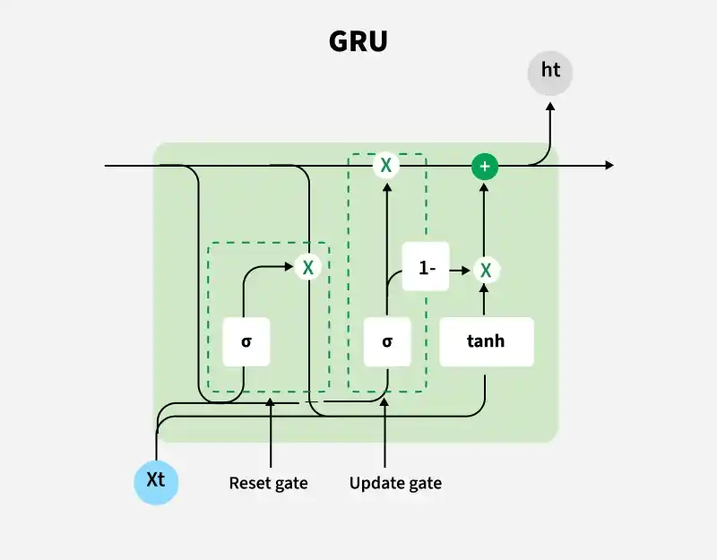
The GRU consists of two main gates:
- Update Gate (zt): Controls how much of the previous hidden state should be carried forward to the current time step. It helps the network decide what information to keep from the past.
- Reset Gate (rt): Determines how much of the previous hidden state should be ignored when computing the new candidate hidden state. It helps the network decide what past information to forget.
These gates allow GRU to control the flow of information in a more efficient manner compared to traditional RNNs which solely rely on hidden state.
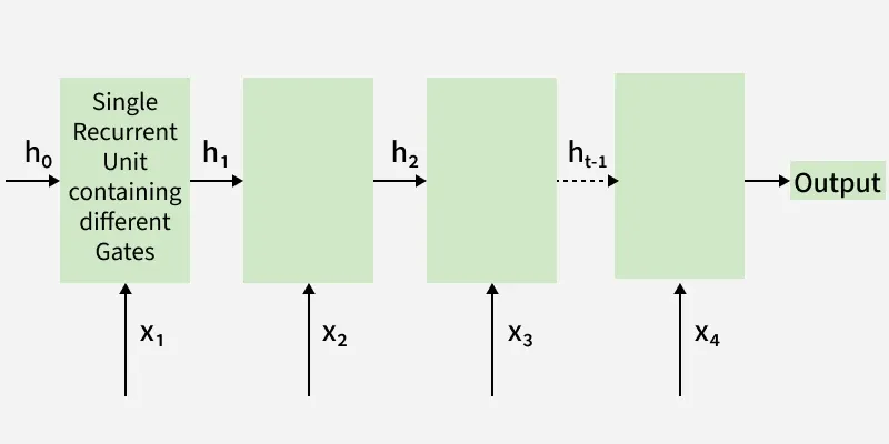
How it Works
The GRU processes sequences by selectively keeping or forgetting information at each time step. Its update and reset gates work together to efficiently capture long-term dependencies in the data.
1. Reset Gate
The reset gate determines how much of the previous hidden state should be forgotten
r_t = \sigma \big( W_r \cdot [h_{t-1}, x_t] \big)
h_{t-1} : Previous hidden statex_{t} : Input at time step tW_{r} : Weight matrix for reset gate\sigma : Sigmoid function that outputs values between 0 and 1
The operation
[h_{t-1},x_{t}] represents concatenation of the previous hidden stateh_{t-1} and the current inputx_{t}
2. Update Gate
The update gate decides how much of the previous hidden state should be carried forward to the current step
z_t = \sigma \big( W_z \cdot [h_{t-1}, x_t] \big)
where
3. Candidate Hidden State
The candidate hidden state represents the potential new information for the current step
{h}_t^{'} = \tanh \big( W_h \cdot [r_t \cdot h_{t-1}, x_t] \big)
where
Here we combines selected past information and current input to form the new candidate
4. Final Hidden State
The final hidden state is a combination of the previous hidden state and the candidate hidden state, controlled by the update gate:
h_t = (1 - z_t) . h_{t-1} + z_t . {h}_t^{'}
The final hidden state
Step By Step Implementation
Here we implement GRU in R Programming Language.
Step 1: Install and Load Necessary Libraries
We will use the keras library, which provides a high-level API for building and training deep learning models in R. Ensure you have the keras library installed and loaded.
install.packages("keras")
install.packages("tensorflow")
library(keras)
library(tensorflow)
Step 2: Prepare Your Data
Here we create a simple time series dataset. We will generate a sine wave and use it for training our GRU model.
# Example data: sine wave
set.seed(42)
time_steps <- 100
data <- sin(seq(0, 10, length.out = time_steps)) + rnorm(time_steps, sd = 0.1)

# Normalize data
data <- scale(data)

# Prepare training data
x_train <- data[1:(time_steps - 1)]
y_train <- data[2:time_steps]

x_train <- array_reshape(x_train, c(length(x_train), 1, 1))
y_train <- array_reshape(y_train, c(length(y_train), 1))
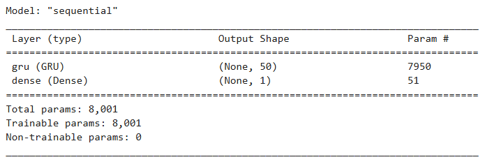
Step 3: Build the GRU Model
We will use the keras library to define and compile the GRU model.
model <- keras_model_sequential() %>%
  layer_gru(units = 50, input_shape = c(1, 1), return_sequences = FALSE) %>%
  layer_dense(units = 1)

model %>% compile(
  loss = 'mean_squared_error',
  optimizer = 'adam'
)
summary(model)
Output:
Step 4: Train the GRU Model
Train the model using the training data.
history <- model %>% fit(
  x_train, y_train,
  epochs = 100,
  batch_size = 1,
  validation_split = 0.2,
  verbose = 1
)
history
Output:
Final epoch (plot to see history):
loss: 0.05499
val_loss: 0.04849
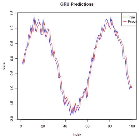
Step 5: Make Predictions
Use the trained model to make predictions.
predictions <- model %>% predict(x_train)

# Plot predictions
plot(data, type = 'l', col = 'blue', main = 'GRU Predictions')
lines(c(NA, as.numeric(predictions)), col = 'red')
legend('topright', legend = c('True', 'Predicted'), col = c('blue', 'red'), lty = 1)
Output:
Download full code from here
GRU vs LSTM
GRUs and Long Short-Term Memory (LSTM) networks are both designed to handle sequential data and long-term dependencies, but they differ in structure and computational efficiency.
Feature | GRU | LSTM |
|---|---|---|
Number of Gates | 2 (Update and Reset) | 3 (Input, Forget, Output) |
Memory Cell | No separate cell state uses hidden state only | Uses separate cell state and hidden state |
Complexity | Simpler, fewer parameters | More complex, more parameters |
Training Speed | Faster due to fewer parameters | Slower due to more gates |
Performance | Often performs better or similar | Can overfit on smaller datasets |
Long-Term Memory Handling | Good, but slightly less flexible | Excellent due to separate cell state |
Limitations
- Less Flexible Memory Control: Unlike LSTMs, GRUs do not have a separate cell state which can limit their ability to capture very long-term dependencies in complex sequences.
- Performance on Extremely Long Sequences: GRUs may struggle with very long sequences compared to LSTMs in tasks like long document text generation or extended time-series forecasting.
- Sensitivity to Hyperparameters: GRUs require careful tuning of parameters such as learning rate, number of units and sequence length to achieve optimal performance.
- Not Always Superior: While faster and lighter than LSTMs, GRUs do not always outperform LSTMs in some datasets, LSTMs may give better results.
- Limited Interpretability: Like most RNNs, GRUs act as a black box, making it difficult to interpret which features or time steps are most influential.