Aquileo | Gradient Descent Algorithm in Machine Learning

Gradient Descent is an optimization algorithm used to minimize the error of a machine learning model by updating parameters in the direction of decreasing loss.

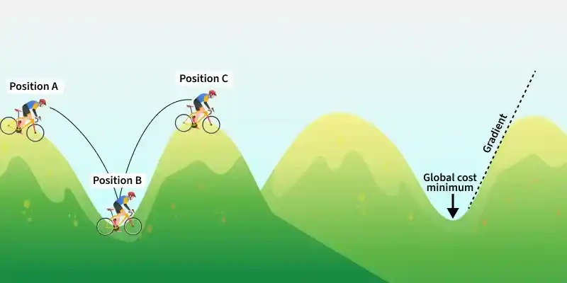
gradient_intuition — Try to reach global minima where error is minimum₹

Minimizes the loss or error of a model
Updates parameters step by step using gradients
Helps models like neural networks and regression learn optimal weights
Variants include Batch Gradient Descent, Stochastic Gradient Descent and Mini Batch Gradient Descent

Formula:

\text{General Update Rule:}w = w - \alpha \frac{\partial L}{\partial w} \\b = b - \alpha \frac{\partial L}{\partial b} \\\\\text{where} \\\alpha : learning\ rate \\L : loss\ function \\\frac{\partial L}{\partial w}, \frac{\partial L}{\partial b} : gradients\ of\ loss

1. Linear Regression

Linear Regression is a supervised learning algorithm used to predict continuous numerical values by modeling the relationship between input variables and the output using a best-fit line.

Predicts continuous values (e.g., price, temperature)
Models relationship using a straight line
Minimizes prediction error using Mean Squared Error (MSE)
Simple and widely used regression technique

\hat{y} = wx + b
L = \frac{1}{2n}\sum_{i=1}^n (y_i - \hat{y}_i)^2

Where:

x: input feature
w: weight (slope of the line)
b: bias/intercept
\hat y: predicted output
y_i : true target value
n: number of samples
L: MSE loss

Role of Gradient Descent

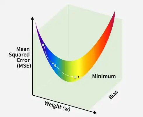
Gradient Descent helps the Linear Regression model find the best values of weight w and bias b so that the prediction error becomes as small as possible. It starts with random values and gradually adjusts them in the direction that reduces the loss.

mean_squared_error_mse_ — Gradient Descent

Calculates how the loss changes with respect to weight w and bias b
Updates these parameters step by step to reduce prediction error
Repeats the process until the loss becomes very small and the best line is found

Implementation

Creates a dataset: Generates 200 sample data points with some random noise.
Initializes parameters: Starts with initial values for weight and bias, and sets the learning rate and number of iterations.
Trains the model: In each iteration, the model makes predictions, calculates the error and updates the parameters using Gradient Descent.
Tracks the loss: Stores the loss value in every iteration to observe how the error changes.
Plots the loss graph: Shows how the error decreases over iterations.
Plots the fitted line: Displays the data points along with the final regression line learned by the model.

Python

import numpy as np
import matplotlib.pyplot as plt
np.random.seed(0)

n = 200
X = np.linspace(-3, 3, n).reshape(-1, 1)
y = 2 * X.ravel() - 0.3 + 0.7 * np.random.randn(n)

w, b = 0.0, 0.0
lr = 0.05
epochs = 200
losses = []

for _ in range(epochs):
    preds = w * X.ravel() + b
    err = preds - y
    loss = (err**2).mean() / 2
    losses.append(loss)
    dw = (X.ravel() * err).mean()
    db = err.mean()
    w -= lr * dw
    b -= lr * db

plt.figure()
plt.plot(losses, color="green")
plt.title("Linear Regression — Loss (MSE)")
plt.xlabel("Epoch")
plt.ylabel("Loss")
plt.grid(True)
plt.show()

plt.figure()
plt.scatter(X, y, color="lightgreen")
idx = np.argsort(X.ravel())
plt.plot(X[idx], (w * X + b)[idx], color="green", linewidth=2)
plt.title("Linear Regression — Fitted Line")
plt.xlabel("x")
plt.ylabel("y")
plt.grid(True)
plt.show()

Output:

2. Logistic Regression

Logistic Regression is a supervised learning algorithm used for binary classification, predicting the probability that a data point belongs to a specific class.

Used for binary classification tasks
Outputs probabilities between 0 and 1 using the sigmoid function
Converts probabilities into class labels (e.g., 0 or 1)
Trained by minimizing binary cross-entropy loss
Simple and effective for classification problems

\sigma(z) = \frac{1}{1 + e^{-z}}
L = -\frac{1}{n}\sum_{i=1}^{n} \left( y_i\ln(\hat{p}_i) + (1 - y_i)\ln(1 - \hat{p}_i) \right)

Where:

𝑧=𝑤⋅𝑥+𝑏 : linear combination
\sigma(z): sigmoid output
\hat P_i : predicted probability
y_i \in \{0,1\}: actual label
n: number of samples
L: cross-entropy loss

Role of Gradient Descent

Gradient descent helps logistic regression find optimal parameter values by reducing prediction error over time.

Computes how cross-entropy loss changes with respect to model parameters
Updates parameters step by step to improve probability predictions
Iteratively reduces loss until the model converges to better performance

Implementation

Creates a dataset: Generates sample data with two classes.
Trains the model using Gradient Descent: The model predicts probabilities, calculates the error using cross entropy loss and updates the weights and bias to reduce the loss.
Shows learning progress: Plots a graph of loss vs iterations to show how the error decreases during training.
Shows the final classification boundary: Displays the data points and the decision boundary learned by the model.

Python

import numpy as np
import matplotlib.pyplot as plt
from sklearn.datasets import make_blobs
np.random.seed(1)

X, y = make_blobs(n_samples=300, centers=2, cluster_std=1.2)
w = np.zeros(X.shape[1])
b = 0.0
lr = 0.2
losses = []

def sigmoid(z): return 1 / (1 + np.exp(-z))

for _ in range(300):
    z = X.dot(w) + b
    p = sigmoid(z)
    loss = -(y * np.log(p + 1e-12) + (1 - y) * np.log(1 - p + 1e-12)).mean()
    losses.append(loss)
    dw = X.T.dot(p - y) / len(X)
    db = (p - y).mean()
    w -= lr * dw
    b -= lr * db

plt.figure()
plt.plot(losses, color="green")
plt.title("Logistic Regression — Loss")
plt.xlabel("Epoch")
plt.ylabel("Loss")
plt.grid(True)
plt.show()

xx, yy = np.meshgrid(
    np.linspace(X[:, 0].min() - 1, X[:, 0].max() + 1, 200),
    np.linspace(X[:, 1].min() - 1, X[:, 1].max() + 1, 200)
)
grid = np.c_[xx.ravel(), yy.ravel()]
probs = sigmoid(grid.dot(w) + b).reshape(xx.shape)

plt.figure()
plt.contourf(xx, yy, probs, 20, cmap="Greens")
plt.scatter(X[:, 0], X[:, 1], c=y, cmap="Greens", edgecolor="black")
plt.title("Logistic Regression — Decision Boundary")
plt.xlabel("x1")
plt.ylabel("x2")
plt.show()

Output:

3. Softmax Regression

Softmax Regression is an extension of logistic regression used for multi-class classification, predicting probabilities across multiple classes.

Used for multi-class classification problems
Outputs a probability distribution over all classes
Uses the softmax function to convert scores into probabilities
Selects the class with the highest probability as the prediction
Trained by minimizing categorical cross-entropy loss

\hat{p}_{i,k} = \frac{e^{z_{i,k}}}{\sum_{j=1}^{K} e^{z_{i,j}}}
L = -\frac{1}{n}\sum_{i=1}^{n}\sum_{k=1}^{K} y_{i,k}\ln(\hat{p}_{i,k})

Where:

z_{i,k}: score(logit) for class k for sample i
\hat P_{i,k}: probability that sample i belongs to class k
K: number of classes
y_{i,k}: one-hot encoded true label
n: number of samples
L: multiclass cross-entropy loss

Role of Gradient Descent

Gradient descent helps the softmax regression model learn optimal parameters by reducing prediction error and improving class probabilities.

Computes how multiclass cross-entropy loss changes with respect to the weights
Updates weights step by step to improve probability of the correct class
Iteratively reduces loss until the model achieves better performance

Implementation

Creates a dataset: Generates sample data with three different classes.
Trains the model using Gradient Descent: The model calculates class probabilities using the softmax function, computes the error using cross entropy loss and updates the weights and bias to reduce the loss.
Shows learning progress: Plots a graph of loss vs iterations to show how the error decreases during training.
Shows the final class regions: Displays the data points and the regions learned by the model for each class.

Python

import numpy as np
import matplotlib.pyplot as plt
from sklearn.datasets import make_blobs
np.random.seed(2)

X, y = make_blobs(n_samples=450, centers=3, cluster_std=1.5)
K = 3

W = np.zeros((X.shape[1], K))
b = np.zeros(K)
lr = 0.2
epochs = 300
losses = []

def softmax(z):
    z -= z.max(axis=1, keepdims=True)
    expz = np.exp(z)
    return expz / expz.sum(axis=1, keepdims=True)

for _ in range(epochs):
    logits = X.dot(W)+b
    probs = softmax(logits)
    Y = np.zeros_like(probs); Y[np.arange(len(y)), y] = 1
    loss = -np.sum(Y*np.log(probs+1e-12))/len(X)
    losses.append(loss)
    dW = X.T.dot(probs-Y)/len(X)
    db = (probs-Y).mean(axis=0)
    W -= lr*dW
    b -= lr*db

plt.figure()
plt.plot(losses, color="green")
plt.title("Softmax Regression — Loss")
plt.xlabel("Epoch")
plt.ylabel("Loss")
plt.grid(True)
plt.show()

xx, yy = np.meshgrid(
    np.linspace(X[:,0].min()-1, X[:,0].max()+1, 300),
    np.linspace(X[:,1].min()-1, X[:,1].max()+1, 300)
)
grid = np.c_[xx.ravel(), yy.ravel()]
preds = np.argmax(softmax(grid.dot(W)+b), axis=1).reshape(xx.shape)

plt.figure()
plt.contourf(xx, yy, preds, K, cmap="Greens")
plt.scatter(X[:,0], X[:,1], c=y, cmap="Greens", edgecolor="black")
plt.title("Softmax Regression — Class Regions")
plt.xlabel("x1")
plt.ylabel("x2")
plt.show()

Output:

4.Neural Network

A neural network with one hidden layer can learn complex patterns that linear models cannot capture by introducing non-linearity through activation functions.

Uses a hidden layer to model complex relationships
Applies activation functions like ReLU for non-linearity
Uses softmax in the output layer to predict class probabilities
Trained using the backpropagation algorithm

Hidden Layer:

a^{(1)} = \text{ReLU}(W^{(1)}x + b^{(1)})

Output Layer:

\hat{y} = \text{softmax}(W^{(2)}a^{(1)} + b^{(2)})

Loss:

L = -\sum_{k=1}^{K} y_k \ln(\hat{y}_k)

Where:

W^{(1)},W^{(2)}: weight matrices
b^{(1)},b^{(2)}: bias vectors
a^{(1)}: hidden layer activations
x: input vector
\hat y: softmax output probabilities
y_k: true class label (one-hot)
K: number of classes
L: cross-entropy loss

Role of Gradient Descent

Gradient descent helps a neural network learn optimal weights by reducing prediction error, working together with backpropagation to improve performance.

Uses gradients from backpropagation to update weights in each layer
Adjusts weights step by step to reduce prediction error
Iteratively improves learning until the model captures better patterns

Implementation

Creates the dataset and neural network: Generates data with three classes and builds a neural network with one hidden layer.
Trains the model: The network makes predictions, calculates the loss and updates the weights using backpropagation and Gradient Descent.
Shows the results: Plots the training loss over epochs and displays the decision regions learned by the neural network.

Python

import numpy as np
import matplotlib.pyplot as plt
from sklearn.datasets import make_blobs
np.random.seed(3)

X, y = make_blobs(n_samples=450, centers=3, cluster_std=1.5)
K = 3
D = X.shape[1]
H = 32

W1 = np.random.randn(D, H) * np.sqrt(2 / D)
b1 = np.zeros(H)
W2 = np.random.randn(H, K) * np.sqrt(2 / H)
b2 = np.zeros(K)

lr = 0.05
epochs = 200
batch = 64
losses = []

relu = lambda z: np.maximum(0, z)

def softmax(z):
    z -= z.max(axis=1, keepdims=True)
    expz = np.exp(z)
    return expz / expz.sum(axis=1, keepdims=True)

for _ in range(epochs):
    idx = np.random.permutation(len(X))
    Xs, Ys = X[idx], y[idx]
    for i in range(0, len(Xs), batch):
        xb = Xs[i:i + batch]
        yb = Ys[i:i + batch]
        z1 = xb.dot(W1) + b1
        a1 = relu(z1)
        logits = a1.dot(W2) + b2
        probs = softmax(logits)
        Yb = np.zeros_like(probs)
        Yb[np.arange(len(yb)), yb] = 1
        dlog = (probs - Yb) / len(yb)
        dW2 = a1.T.dot(dlog)
        db2 = dlog.sum(axis=0)
        da1 = dlog.dot(W2.T)
        dz1 = da1 * (z1 > 0)
        dW1 = xb.T.dot(dz1)
        db1 = dz1.sum(axis=0)
        W2 -= lr * dW2
        b2 -= lr * db2
        W1 -= lr * dW1
        b1 -= lr * db1

    logits_full = relu(X.dot(W1) + b1).dot(W2) + b2
    pf = softmax(logits_full)
    Yf = np.zeros_like(pf)
    Yf[np.arange(len(y)), y] = 1
    losses.append(-(Yf * np.log(pf + 1e-12)).mean())

plt.figure()
plt.plot(losses, color="green")
plt.title("Neural Network — Loss")
plt.xlabel("Epoch")
plt.ylabel("Loss")
plt.grid(True)
plt.show()

xx, yy = np.meshgrid(
    np.linspace(X[:, 0].min() - 1, X[:, 0].max() + 1, 300),
    np.linspace(X[:, 1].min() - 1, X[:, 1].max() + 1, 300)
)
grid = np.c_[xx.ravel(), yy.ravel()]
pred = np.argmax(softmax(relu(grid.dot(W1) + b1).dot(W2) + b2),
                 axis=1).reshape(xx.shape)

plt.figure()
plt.contourf(xx, yy, pred, K, cmap="Greens")
plt.scatter(X[:, 0], X[:, 1], c=y, cmap="Greens", edgecolor="black")
plt.title("Neural Network — Decision Regions")
plt.xlabel("x1")
plt.ylabel("x2")
plt.show()

Output:

5. Support Vector Machine

A Support Vector Machine is a supervised learning algorithm used for classification and regression that finds the best boundary to separate data points.

Creates a decision boundary (hyperplane) to separate classes
Maximizes the margin between different classes
Uses support vectors (critical data points) to define the boundary
Applies hinge loss to penalize incorrect or close predictions

L = \frac{1}{2} \|w\|^2 + C \cdot \frac{1}{n} \sum_{i=1}^{n} \max(0, 1 - y_i (w \cdot x_i + b))

Where:

w: weight vector
b: bias term
x: input
y \in \{-1,+1\}: class label
C: regularization strength
max(0,1−y(w⋅x+b)): hinge loss
L: total SVM objective

Role of Gradient Descent

Gradient Descent helps the SVM model find the best parameters so that the classification boundary separates the classes as clearly as possible. It adjusts the parameters by reducing hinge loss and improving the margin between classes.

Updates the model parameters to reduce hinge loss
Adjusts the boundary when points are misclassified or too close to it
Repeats the process to improve the margin and classification accuracy

Implementation

Creates a dataset: Generates sample data with two classes and converts labels into values suitable for SVM training.
Trains the SVM using Gradient Descent: Calculates hinge loss, updates the model parameters step by step and improves the decision boundary during training.
Shows the results: Plots the objective value over iterations and displays the final decision boundary separating the two classes.

Python

import numpy as np
import matplotlib.pyplot as plt
from sklearn.datasets import make_blobs
np.random.seed(4)

X, y_binary = make_blobs(n_samples=300, centers=2, cluster_std=1.2)
y = 2 * y_binary - 1

w = np.zeros(X.shape[1])
b = 0.0
lr = 0.01
C = 1.0
epochs = 500
losses = []

for _ in range(epochs):
    margins = y * (X.dot(w) + b)
    hinge = np.maximum(0, 1 - margins)
    loss = 0.5 * np.dot(w, w) + C * hinge.mean()
    losses.append(loss)
    mask = margins < 1
    if mask.any():
        dw = w - (C / len(X)) * X[mask].T.dot(y[mask])
        db = -(C / len(X)) * y[mask].sum()
    else:
        dw = w
        db = 0.0
    w -= lr * dw
    b -= lr * db

plt.figure()
plt.plot(losses, color="green")
plt.title("Linear SVM (hinge) — Objective")
plt.xlabel("Epoch")
plt.ylabel("Objective")
plt.grid(True)
plt.show()

xx, yy = np.meshgrid(
    np.linspace(X[:, 0].min() - 1, X[:, 0].max() + 1, 200),
    np.linspace(X[:, 1].min() - 1, X[:, 1].max() + 1, 200)
)
grid = np.c_[xx.ravel(), yy.ravel()]
scores = grid.dot(w) + b

plt.figure()
plt.contourf(xx, yy, (scores.reshape(xx.shape) > 0).astype(int), cmap="Greens")
plt.scatter(X[:, 0], X[:, 1], c=y_binary, cmap="Greens",
            edgecolor="black", alpha=0.85)
plt.title("Linear SVM — Decision Boundary (approx)")
plt.xlabel("x1")
plt.ylabel("x2")
plt.show()

Output:

6. Matrix Factorization

Matrix Factorization is used in recommender systems to find hidden patterns in user item ratings. It breaks the rating matrix into smaller latent factors representing user preferences and item features, which are used to predict missing ratings.

Reconstruction:

R \approx P Q^T

Loss:

L = \sum_{(i,j)\in\Omega} (R_{ij} - P_iQ_j^T)^2 + \lambda (\|P\|^2 + \|Q\|^2)

Where:

R: rating matrix
P: user latent matrix
Q: item latent matrix
\Omega : observed user-item pairs
R_{ij}: actual rating
P_iQ^T_j : predicted rating
\lambda: regularization strength
L: reconstruction loss

Role of Gradient Descent

Gradient Descent helps the Matrix Factorization model learn the best user and item factors so that the predicted ratings become closer to the actual ratings. It:

Updates user and item latent vectors using observed ratings
Reduces the difference between predicted and actual ratings
Repeats the process to learn better user and item representations

Implementation

Creates a rating dataset: Generates a user item rating matrix and keeps only some ratings as observed data.
Trains the model using Gradient Descent: Updates user and item latent factors using the observed ratings to reduce prediction error.
Shows learning progress: Plots the loss over epochs to show how the reconstruction error decreases.
Shows the reconstructed matrix: Displays the observed ratings and the reconstructed full matrix learned by the model.

Python

import numpy as np
import matplotlib.pyplot as plt
np.random.seed(5)

n_users, n_items = 30, 25
true_k = 4
P_true = np.random.randn(n_users, true_k)
Q_true = np.random.randn(n_items, true_k)
R_full = P_true.dot(Q_true.T)

mask = np.random.rand(n_users, n_items) < 0.4
R = np.where(mask, R_full + 0.5 * np.random.randn(n_users, n_items), 0.0)

k = 4
P = 0.1 * np.random.randn(n_users, k)
Q = 0.1 * np.random.randn(n_items, k)
lr = 0.01
epochs = 80
reg = 0.1
losses = []

obs = np.argwhere(mask)
for _ in range(epochs):
    np.random.shuffle(obs)
    for i, j in obs:
        pred = P[i].dot(Q[j])
        err = R[i, j] - pred
        dP = -2 * err * Q[j] + 2 * reg * P[i]
        dQ = -2 * err * P[i] + 2 * reg * Q[j]
        P[i] -= lr * dP
        Q[j] -= lr * dQ
    pred_all = P.dot(Q.T)
    diff = mask * (R - pred_all)
    loss = (diff**2).sum() / mask.sum() + reg * (np.sum(P**2) + np.sum(Q**2))
    losses.append(loss)

plt.figure()
plt.plot(losses, color="green")
plt.title("Matrix Factorization — Loss (observed)")
plt.xlabel("Epoch")
plt.ylabel("Loss")
plt.grid(True)
plt.show()

recon = P.dot(Q.T)
plt.figure(figsize=(10, 4))
plt.subplot(1, 2, 1)
plt.imshow(np.where(mask, R, np.nan), aspect='auto', cmap="Greens")
plt.title("Observed Ratings")
plt.xlabel("Item index")
plt.ylabel("User index")
plt.colorbar(shrink=0.6)

plt.subplot(1, 2, 2)
plt.imshow(recon, aspect='auto', cmap="Greens")
plt.title("Reconstructed Matrix")
plt.xlabel("Item index")
plt.ylabel("User index")
plt.colorbar(shrink=0.6)

plt.tight_layout()
plt.show()

Output:

Download code for all implementations from here

Gradient Descent Algorithm in Machine Learning

1. Linear Regression

Role of Gradient Descent

Implementation

2. Logistic Regression

Role of Gradient Descent

Implementation

3. Softmax Regression

Role of Gradient Descent

Implementation

4.Neural Network

Role of Gradient Descent

Implementation

5. Support Vector Machine

Role of Gradient Descent

Implementation

6. Matrix Factorization

Role of Gradient Descent

Implementation

Explore