What are Graph Neural Networks?

Graph Neural Networks (GNNs) are deep learning models designed to work with graph-structured data, where information is represented as nodes and edges. Unlike traditional neural networks that handle fixed-size inputs, GNNs capture relationships, dependencies and interactions between entities.

• They operate on graphs made of nodes and edges.
• Information is passed between connected nodes (neighbors) through message-passing steps.
• Useful for tasks like social network analysis, molecule prediction and recommendation systems.
• They learn both node-level and graph-level patterns.

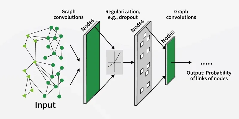
This image shows how a GNN processes a graph node features pass through stacked graph convolution layers with regularization, gradually refining representations until the model outputs predictions such as the probability of links between nodes.

GNN Architectures

Graph Neural Networks can be built in different ways depending on how they aggregate information and update node representations. One of the most commonly used architectures is the Graph Convolutional Network (GCN) which extends the idea of convolution from images to graph structured data.

Graph Convolutional Network (GCN)

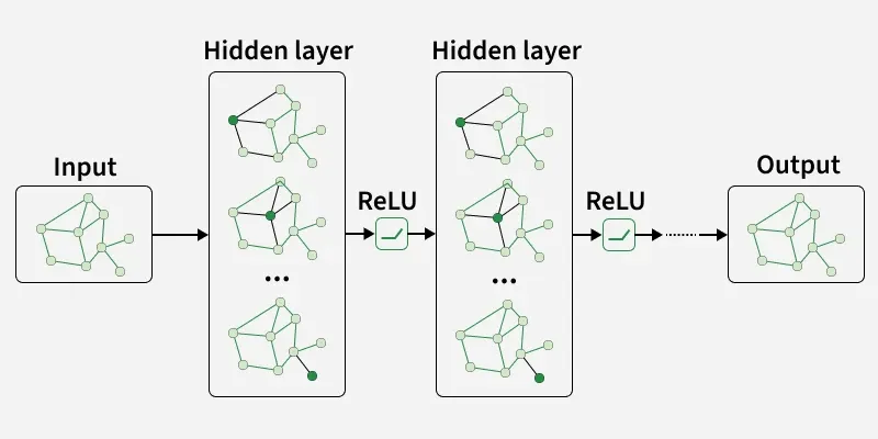
A basic GCN for graph classification usually contains three main layers:

• Convolutional Layer: Aggregates features from each node neighbors.
• Activation Layer: Applies a non linearity like ReLU.
• Output Layer: Produces the final prediction for the graph.

GCNs are easy to implement and efficient for large graphs, but they cannot use edge features and do not perform full message passing, limiting their ability to model complex graph relationships.

Message Passing Neural Networks (MPNNs)

MPNNs overcome these limitations by supporting both node and edge features. In each iteration:

• Nodes collect messages from their neighbors.
• The aggregated information updates each node’s embedding.
• The process repeats for multiple rounds.

MPNNs provide richer representations and support node classification, edge classification and link prediction, making them more flexible and expressive than basic GCNs.

GCNs and MPNNs represent two core ways of processing graph data and together they form GNN architectures.

How Do GNN Work

Graph Neural Networks work by allowing nodes in a graph to share information with their neighbors through a process known as message passing. Since graphs are irregular and unstructured, GNNs organize this data so deep learning models can extract meaningful patterns.

1. Initialization: Each node begins with a feature vector describing its properties such as user attributes or atom characteristics.
2. Message Passing: Nodes share information with their neighbors across layers, allowing each node to learn context from the surrounding graph structure.
3. Update: After aggregation, nodes update their feature vectors using a neural network layer.

GNNs use sparse operations and usually require only a few layers making them efficient for relational and interconnected data.

Types of Graph Neural Networks

Graph Neural Networks come in various forms, each designed to process graph-structured data in a unique way. Different GNN architectures focus on how information is aggregated, propagated or transformed across nodes and edges.

1. Graph Convolutional Networks (GCN)

• Extend the idea of convolution from grid data to graphs.
• Update a node’s representation by aggregating features from its neighbors.
• Capture both local and global graph information through multiple stacked layers.
• Widely used for semi-supervised tasks such as node classification and label prediction.

2. Graph Attention Networks (GAT)

• Introduce an attention mechanism during message passing.
• Assign different importance weights to neighboring nodes based on relevance.
• Better handle graphs with uneven or complex connectivity patterns.
• Useful in social networks, citation graphs and recommendation systems.

3. Graph Recurrent Networks (GRN)

• Combine graph structures with recurrent neural network concepts.
• Designed to handle temporal or evolving graph data.
• Maintain and update hidden states to track changes over time.
• Suitable for dynamic graphs such as traffic flow, communication patterns or social interactions.

4. Spatial based GNN

• Operate directly on the graph’s topology in the spatial domain.
• Pass messages based on the physical or structural neighborhood of each node.
• Intuitive and efficient for large, real-world graphs.

5. Spectral based GNN

• Use spectral graph theory and graph Fourier transforms for convolution.
• Capture global and frequency-based properties of the graph.
• Often used in mathematical or highly structured graph learning tasks.

Step-By-Step Implementation

Step 1: Imports Libraries

We will import pytorch, scikit learn, matplotlib and numpy.

import torch
import torch.nn as nn
import torch.nn.functional as F
import torch.optim as optim

from torch_geometric.datasets import TUDataset
from torch_geometric.data import DataLoader
import torch_geometric.nn as pyg_nn
import torch_geometric.transforms as T
import torch_geometric.utils as pyg_utils

from sklearn.manifold import TSNE
import matplotlib.pyplot as plt
import networkx as nx
import numpy as np

device = torch.device('cuda' if torch.cuda.is_available() else 'cpu')
print("Using device:", device)

Output:

Device: cuda

Step 2 Load the MUTAG dataset

• Uses TUDataset which contains many small graphs.
• Shuffles and splits into 80% train and 20% test.
• NormalizeFeatures scales node features.
• loader_train and loader_test yield batches of graphs.

dataset = TUDataset(root='data/TUDataset', name='MUTAG', use_node_attr=False, transform=T.NormalizeFeatures())

dataset = dataset.shuffle()
n = len(dataset)
n_train = int(0.8 * n)
train_dataset = dataset[:n_train]
test_dataset = dataset[n_train:]

print(f"Loaded MUTAG. Total graphs: {len(dataset)} | Train: {len(train_dataset)} | Test: {len(test_dataset)}")

loader_train = DataLoader(train_dataset, batch_size=64, shuffle=True)
loader_test = DataLoader(test_dataset, batch_size=64, shuffle=False)

Step 3: Define the GNN model

• GINConv is a useful graph aggregator for graph classification.
• num_layers controls message passing depth.
• global_mean_pool pools node embeddings to graph embeddings.
• post_mp is an MLP that converts pooled embedding to class logits.
• loss() returns NLL loss expecting F.log_softmax outputs.

class GNNStack(nn.Module):
    def __init__(self, input_dim, hidden_dim, output_dim, num_layers=3, dropout=0.25):
        super(GNNStack, self).__init__()
        self.num_layers = num_layers
        self.dropout = dropou
        self.convs = nn.ModuleList()
        self.convs.append(pyg_nn.GINConv(nn.Sequential(
            nn.Linear(input_dim, hidden_dim), nn.ReLU(), nn.Linear(hidden_dim, hidden_dim)
        )))
        for _ in range(1, num_layers):
            self.convs.append(pyg_nn.GINConv(nn.Sequential(
                nn.Linear(hidden_dim, hidden_dim), nn.ReLU(), nn.Linear(hidden_dim, hidden_dim)
            )))
        self.lns = nn.ModuleList([nn.LayerNorm(hidden_dim) for _ in range(num_layers - 1)])

        self.post_mp = nn.Sequential(
            nn.Linear(hidden_dim, hidden_dim),
            nn.ReLU(),
            nn.Dropout(dropout),
            nn.Linear(hidden_dim, output_dim)
        )

    def forward(self, data):
        x, edge_index, batch = data.x, data.edge_index, data.batch
        if x is None:
            x = torch.ones((data.num_nodes, 1), device=edge_index.device)

        for i, conv in enumerate(self.convs):
            x = conv(x, edge_index)
            if i != self.num_layers - 1:
                x = F.relu(x)
                x = F.dropout(x, p=self.dropout, training=self.training)
                x = self.lns[i](x)

        emb = x  
        g_emb = pyg_nn.global_mean_pool(emb, batch)
        out = self.post_mp(g_emb)
        return emb, F.log_softmax(out, dim=1)

    def loss(self, pred_logprob, label):
        return F.nll_loss(pred_logprob, label)

Step 4: Instantiate model and optimizer

• input_dim uses dataset node features.
• Move model to device.
• Adam optimizer with small weight decay for regularization.

input_dim = max(1, dataset.num_node_features)
num_classes = dataset.num_classes

model = GNNStack(input_dim=input_dim, hidden_dim=64, output_dim=num_classes, num_layers=3, dropout=0.25).to(device)
optimizer = optim.Adam(model.parameters(), lr=0.01, weight_decay=5e-4)

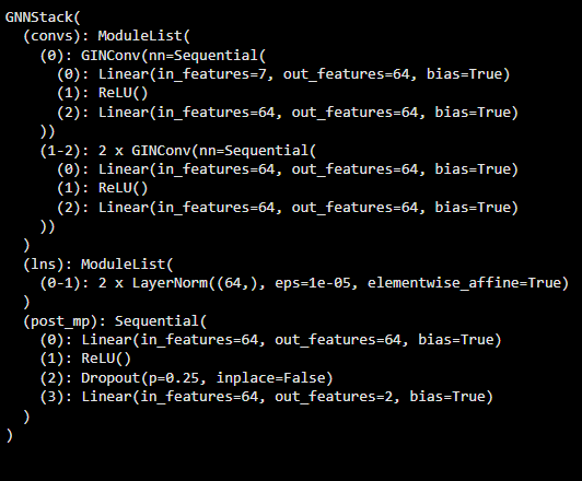
print(model)

Output:

Step 5: Training and evaluation helpers

• train_graph_epoch trains for one epoch across batches.
• Multiply loss by batch.num_graphs to accumulate correctly.
• eval_graph computes accuracy over test batches.
• Functions expect batches moved to device.

def train_graph_epoch(loader):
    model.train()
    total_loss = 0.0
    total_graphs = 0
    for batch in loader:
        batch = batch.to(device)
        optimizer.zero_grad()
        emb, pred = model(batch) 
        loss = model.loss(pred, batch.y)
        loss.backward()
        optimizer.step()
        total_loss += loss.item() * batch.num_graphs
        total_graphs += batch.num_graphs
    return total_loss / total_graphs

@torch.no_grad()
def eval_graph(loader):
    model.eval()
    correct = 0
    total = 0
    for batch in loader:
        batch = batch.to(device)
        emb, pred = model(batch)
        pred_label = pred.argmax(dim=1)
        correct += (pred_label == batch.y).sum().item()
        total += batch.num_graphs
    return correct / total

Step 6: Run training loop & log metrics

Train for num_epochs, store loss and test accuracy lists.

num_epochs = 100
train_losses = []
test_scores = []

for epoch in range(1, num_epochs + 1):
    loss = train_graph_epoch(loader_train)
    acc = eval_graph(loader_test)
    train_losses.append(loss)
    test_scores.append(acc)
    if epoch % 10 == 0 or epoch == 1:
        print(f"[Graph] Epoch {epoch:03d} | Loss: {loss:.4f} | Test Acc: {acc:.4f}")

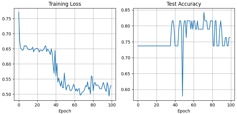
Step 7: Plot training loss and test accuracy

Use these to check convergence and overfitting.

plt.figure(figsize=(10,4))
plt.subplot(1,2,1)
plt.plot(train_losses, label='Train Loss')
plt.xlabel('Epoch'); plt.ylabel('Loss'); plt.title('Training Loss'); plt.grid(True); plt.legend()

plt.subplot(1,2,2)
plt.plot(test_scores, label='Test Accuracy')
plt.xlabel('Epoch'); plt.ylabel('Accuracy'); plt.title('Test Accuracy'); plt.grid(True); plt.legend()

plt.tight_layout()
plt.show()

Output:

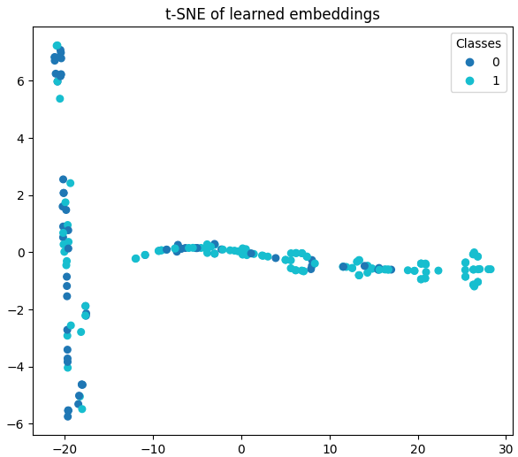
Step 8: Get graph embeddings and t-SNE visualization

• Run model over all graphs, pool node embeddings to get graph-level embeddings.
• Apply t-SNE to reduce to 2D and scatter-plot colored by class.
• Clusters indicate separability of learned graph representations.

@torch.no_grad()
def get_graph_embeddings_and_labels():
    model.eval()
    all_embs = []
    all_labels = []
    loader = DataLoader(dataset, batch_size=64, shuffle=False)
    for batch in loader:
        batch = batch.to(device)
        emb, pred = model(batch)   
        g_emb = pyg_nn.global_mean_pool(emb, batch.batch)
        all_embs.append(g_emb.cpu())
        all_labels.append(batch.y.cpu())
    embs = torch.cat(all_embs, dim=0).numpy()
    labels = torch.cat(all_labels, dim=0).numpy()
    return embs, labels

embs, labels = get_graph_embeddings_and_labels()
print("Embeddings shape:", embs.shape, "Labels shape:", labels.shape)

tsne = TSNE(n_components=2, random_state=42, perplexity=20)
emb2 = tsne.fit_transform(embs)

plt.figure(figsize=(7,6))
scatter = plt.scatter(emb2[:,0], emb2[:,1], c=labels, cmap='tab10', s=40)
plt.legend(*scatter.legend_elements(), title="Classes")
plt.title('t-SNE of learned graph embeddings')
plt.show()

Output:

You can download full code from here.

Applications

• Social Network Analysis: Used to predict user behavior, community detection, friend recommendations and influence modeling.
• Molecular Chemistry and Drug Discovery: Helps predict molecular properties, drug target interactions and protein structure by treating molecules as graphs.
• Knowledge Graph Completion: Used to infer missing relations between entities in large knowledge bases.
• Recommendation Systems: Models user item interactions as graphs for better recommendations.
• Traffic and Transportation Networks: Predicts traffic flow, congestion patterns and route optimization using dynamic graph data.

Advantages

• Handles Irregular Data: Works naturally with non-Euclidean structures like social networks and molecules.
• Learns Node Relationships: Aggregates neighbor information to build meaningful node embeddings.
• Scales Across Graph Sizes: Works on small and large graphs without changing the model.
• Flexible Predictions: Supports node-level, edge-level and whole-graph prediction tasks.
• Great for Semi-Supervised Learning: Performs well even when only a few nodes have labels.

Limitations

• High Computational Cost: Large graphs require significant memory and processing power.
• Over-Smoothing Problem: When too many GNN layers are stacked, node features become indistinguishable.
• Scalability Challenges: Hard to train on extremely large or dynamic graphs without specialized techniques.
• Dependency on Graph Quality: Poor or noisy graph structure can lead to incorrect learning.
• Long-Range Dependency Modeling: Standard GNNs struggle to capture very distant node relationships without deeper architectures.