Neural Style Transfer with TensorFlow

Neural Style Transfer (NST) is a method in deep learning where the details of one picture are combined with the artistic style of another to create a new image. This process allows you to generate an image that has the subject of the first picture but the art style, colors and textures of the second. In this guide we will explain how NST works and how to apply it using TensorFlow.

Understanding Neural Style Transfer

 Neural Style Transfer or NST involves three different images:

• Content Image: This is the picture with the main subject or scene you want to change. It holds the basic structure and layout you want to keep
• Style Image: the picture with the artistic feel, like colors, textures and patterns. You want to use this style to change how your content image looks.
• Generated Image: The output image that combines the content of the first image with the style of the second.

The process of NST uses a type of computer model called a convolutional neural network (CNN). A well-known CNN often used in NST is called VGG19. This computer model analyzes details and features in both the content and style images. To make the new image the computer model works with a formula known as a loss function. This formula keeps the computer to find the best mix of subject from the content image and the artistic elements from the style image.

To understand the Neural Style Transfer more refer to: Overview of Style Transfer

Implementing Neural Style Transfer with TensorFlow

In implementation of NST we'll use the VGG19 model, pre-trained on the ImageNet dataset to extract features from our images.

Step 1: Import Necessary Libraries

First we import the necessary module like TensorFlow v2 with Keras, NumPy for numerical operations, Matplotlib for data visualisation and Keras-specific components for working with pre-trained models and image processing.

import tensorflow as tf
import numpy as np
import matplotlib.pyplot as plt
import math

from tensorflow.keras.applications.vgg19 import VGG19, preprocess_input
from tensorflow.keras.preprocessing.image import load_img, img_to_array
from tensorflow.keras.models import Model

Step 2: Image processing

Now, we load and process the image using Keras preprocess input in VGG 19. The expand_dims function adds a dimension to represent a number of images in the input. This preprocess_input function used in VGG 19 converts the input RGB to BGR images and centre these values around 0 according to ImageNet data.

def load_and_process_image(image_path):
    img = load_img(image_path)

    img = img_to_array(img)
    img = preprocess_input(img)
    img = np.expand_dims(img, axis=0)
    return img

Now, we define the deprocess function that takes the input image and perform the inverse of preprocess_input function that we imported above. To display the unprocessed image we also define a display function.

def deprocess(img):
    img[:, :, 0] += 103.939
    img[:, :, 1] += 116.779
    img[:, :, 2] += 123.6
    img = img[:, :, ::-1]

    img = np.clip(img, 0, 255).astype('uint8')
    return img


def display_image(image):
    if len(image.shape) == 4:
        img = np.squeeze(image, axis=0)

    img = deprocess(img)

    plt.grid(False)
    plt.xticks([])
    plt.yticks([])
    plt.imshow(img)
    return

Now we use the above function to display the style and content images

content_img = load_and_process_image(content_path)
display_image(content_img)

style_img = load_and_process_image(style_path)
display_image(style_img)

 
Output:

Step 3: Model Initialization

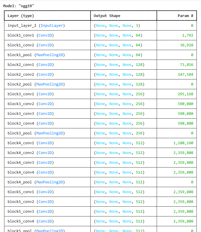
Now we initialize the VGG model with ImageNet weights we will also remove the top layers and make it non-trainable. We use VGG19 to extract image features.

• include_top=False removes the classification head.
• We freeze the model to use it as a fixed feature extractor.

model = VGG19(
    include_top=False,
    weights='imagenet'
)

model.trainable = False

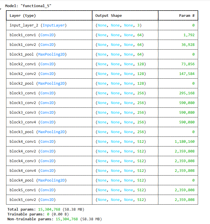
model.summary()

Output:

Step 4: Content Model defining

Now we define the content and style model using Keras.Model API. The content model takes the image as input and output the feature map from "block5_conv1" from the above VGG model.

content_layer = 'block5_conv2'
content_model = Model(
    inputs=model.input,
    outputs=model.get_layer(content_layer).output
)
content_model.summary()

 Output:

Step 5: Style Model defining:

Now, we define the content and style model using Keras.Model API. The style model takes an image as input and output the feature map from "block1_conv1, block3_conv1 and block5_conv2" from the above VGG model. We use multiple layers for style to capture texture patterns at different scales. Each layer captures style at different levels of abstraction like edges, patterns and textures.

style_layers = [
    'block1_conv1',
    'block3_conv1',
    'block5_conv1'
]
style_models = [Model(inputs=model.input,
                      outputs=model.get_layer(layer).output) for layer in style_layers]

Content Loss: Now we define the content loss function it will take the feature map of generated and real images and calculate the mean square difference between them.

def content_loss(content, generated):
    a_C = content_model(content)
    a_G = content_model(generated)  # Add this line to compute a_G
    loss = tf.reduce_mean(tf.square(a_C - a_G))
    return loss

Gram Matrix: Now we define the gram matrix function. This function also takes the real and generated images as the input of the model and calculates gram matrices of them before calculate the style loss weighted to different layers.

def gram_matrix(A):
    channels = int(A.shape[-1])
    a = tf.reshape(A, [-1, channels])
    n = tf.shape(a)[0]
    gram = tf.matmul(a, a, transpose_a=True)
    return gram / tf.cast(n, tf.float32)


weight_of_layer = 1. / len(style_models)

Style Loss: The function style_cost defined by this code determines the style loss between a generated image and a style image that is supplied. In neural style transfer algorithms style loss is frequently employed to create an image that blends the content of two different images with their styles.

def style_cost(style, generated):
    J_style = 0

    for style_model in style_models:
        a_S = style_model(style)
        a_G = style_model(generated)
        GS = gram_matrix(a_S)
        GG = gram_matrix(a_G)
        content_cost = tf.reduce_mean(tf.square(GS - GG))
        J_style += content_cost * weight_of_layer

    return J_style

Content Loss: The content loss between a style image and a generated image is determined by the function content_cost, which is defined in this code. To make sure that the generated image preserves the original image's content, neural style transfer algorithms frequently employ content loss.

def content_cost(style, generated):
    J_content = 0

    for style_model in style_models:
        a_S = style_model(style)
        a_G = style_model(generated)
        GS = gram_matrix(a_S)
        GG = gram_matrix(a_G)
        content_cost = tf.reduce_mean(tf.square(GS - GG))
        J_content += content_cost * weight_of_layer

    return J_content

Step 6: Training Function

In this step we define the training_loop function that optimizes the generated image using both content and style losses. It begins by loading and preprocessing the content and style images then initializes the generated image as a trainable variable.

• GradientTape watches changes in the generated image.
• J_content: difference in content features.
• J_style: difference in style (Gram matrices).
• J_total: weighted combination using a and b.

generated_images = []


def training_loop(content_path, style_path, iterations=50, a=10, b=1000):

    content = load_and_process_image(content_path)
    style = load_and_process_image(style_path)
    generated = tf.Variable(content, dtype=tf.float32)

    opt = tf.keras.optimizers.Adam(learning_rate=0.7)

    best_cost = math.inf
    best_image = None
    for i in range(iterations):
        start_time_cpu = time.process_time()
        start_time_wall = time.time()
        with tf.GradientTape() as tape:
            J_content = content_cost(style, generated)
            J_style = style_cost(style, generated)
            J_total = a * J_content + b * J_style

        grads = tape.gradient(J_total, generated)
        opt.apply_gradients([(grads, generated)])

        end_time_cpu = time.process_time()  
        end_time_wall = time.time()  
        cpu_time = end_time_cpu - start_time_cpu  
        wall_time = end_time_wall - start_time_wall  

        if J_total < best_cost:
            best_cost = J_total
            best_image = generated.numpy()

        print("CPU times: user {} µs, sys: {} ns, total: {} µs".format(
          int(cpu_time * 1e6),
          int(( end_time_cpu - start_time_cpu) * 1e9),
          int((end_time_cpu - start_time_cpu + 1e-6) * 1e6))
             )
        
        print("Wall time: {:.2f} µs".format(wall_time * 1e6))
        print("Iteration :{}".format(i))
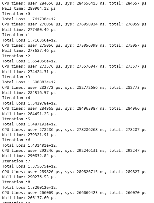
        print('Total Loss {:e}.'.format(J_total))
        generated_images.append(generated.numpy())

    return best_image

Step 7: Model Training

Now, we train our model using the training function we defined above.

final_img = training(content_path, style_path)

Output:

Step 8: Model Prediction

In the final step, we plot the final and intermediate results.

plt.figure(figsize=(12, 12))

for i in range(10):
    plt.subplot(4, 3, i + 1)
    display_image(generated_images[i+39])
plt.show()

display_image(final_img)

Output:

This output shows the last 10 generated images during Neural Style Transfer where the content (dog) is preserved and style patterns are gradually applied. Each image reflects slight improvements in blending style with content across iterations.

Complete Code : click here