Fourier Transform is a mathematical technique used to analyze the frequency components of an image. It converts an image from the spatial domain to the frequency domain, making it useful for image filtering, compression, enhancement, and feature extraction.
- Low-frequency components represent smooth regions and overall image structure.
- High-frequency components represent edges, textures, and fine details.
The continuous Fourier Transform is given by:
F(u,v)=\int_{-\infty}^{\infty}\int_{-\infty}^{\infty}f(x,y)e^{-j2\pi(ux+vy)}dxdy
Steps to find the Fourier Transform of an image
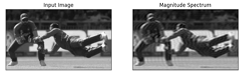
In this program, we will find the Discrete Fourier Transform (DFT) of an input image using OpenCV. The frequency components are processed and the resulting magnitude spectrum is displayed to visualize the image in the frequency domain.
Input Image:

Step 1: Import the Required Libraries
Importing NumPy for numerical operations, OpenCV for image processing, and Matplotlib for visualization.
import numpy as np
import cv2
from matplotlib import pyplot as plt
Step 2: Load the Image
Loading the input image in grayscale mode using the cv2.imread() function, as Fourier Transform is typically applied to grayscale images.
image_path = r"Dhoni-dive_165121_730x419-m.jpg"
image = cv2.imread(image_path, 0)
Step 3: Compute the Discrete Fourier Transform
Converting the image from the spatial domain to the frequency domain using the cv2.dft() function.
DFT = cv2.dft(np.float32(image),
              flags=cv2.DFT_COMPLEX_OUTPUT)
Step 4: Shift the Zero-Frequency Component to the Center
A square mask is created around the center of the spectrum to preserve low-frequency components while suppressing high-frequency components.
shift = np.fft.fftshift(DFT)
row, col = image.shape
center_row, center_col = row // 2, col // 2
Step 5: Apply the Mask and Perform Inverse Shift
The mask is applied to the shifted spectrum. The modified spectrum is then shifted back before performing the inverse transform.
mask = np.zeros((row, col, 2), np.uint8)
mask[center_row - 30:center_row + 30, center_col - 30:center_col + 30] = 1
Step 6: Compute the Inverse DFT and Magnitude Spectrum
The inverse DFT reconstructs the image from the filtered frequency spectrum. The magnitude is calculated to visualize the intensity of the reconstructed image.
imageThen = cv2.idft(fft_ifft_shift) imageThen = cv2.magnitude( imageThen[:, :, 0], imageThen[:, :, 1] )
Step 7: Display the Results
Finally, displaying the original image and the resulting magnitude spectrum using Matplotlib.
plt.figure(figsize=(10,10))
plt.subplot(121), plt.imshow(image, cmap='gray')
plt.title('Input Image'), plt.xticks([]), plt.yticks([])
plt.subplot(122), plt.imshow(imageThen, cmap='gray')
plt.title('Magnitude Spectrum'), plt.xticks([]), plt.yticks([])
plt.show()
Output: