Lasso Regression (Least Absolute Shrinkage and Selection Operator) is a linear regression technique with L1 regularization that improves model generalization by adding a penalty. This penalty not only controls overfitting but also performs automatic feature selection by shrinking some coefficients exactly to zero, making Lasso useful in high-dimensional datasets where interpretability and sparsity are important.
- Uses L1 regularization to reduce overfitting
- Encourages sparse models (zero coefficients)
- Automatically performs feature selection
- Useful for high‑dimensional datasets
Note: L1 regularization adds the sum of absolute values of model weights to the loss function, encouraging sparsity by pushing some weights exactly to zero.
Bias–Variance Tradeoff
The Bias–Variance Tradeoff describes the balance between a model’s simplicity and its ability to generalize to unseen data. In machine learning, reducing bias often increases variance and vice versa, so finding the right balance is important for building accurate models.
Lasso Regression directly influences the bias–variance tradeoff through its regularization strength (λ or α).
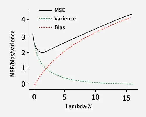
Low λ (weak regularization)
- Model closely fits training data
- Means low bias and high variance
- Risk of overfitting
High λ (strong regularization)
- Coefficients heavily shrunk or removed
- Means higher bias and lower variance
- Better generalization
How Lasso balances this tradeoff
- Penalization reduces variance by simplifying the model
- Feature elimination may increase bias slightly
- Net effect is often lower test error
Working of Lasso Regression
Let's see the working:
1. Base Linear Model
Lasso begins with a standard linear regression setup where the target variable is predicted as a weighted sum of input features. Without regularization, this model can overfit when the number of predictors is large.
2. L1-Regularized Objective Function
\sum_{i=1}^{n} (y_i - \hat{y}_i)^2 + \lambda \sum_{j=1}^{p} |w_j|
- First term measures prediction error
- Second term penalizes absolute coefficient values
- λ determines how strongly coefficients are constrained
3. Coefficient Shrinkage
- As λ increases, coefficients are gradually reduced
- Less important features receive stronger shrinkage
- Some coefficients reach exactly zero
4. Embedded Feature Selection
- Zero-valued coefficients mean features are discarded
- No separate feature selection step is needed
- Results in compact and interpretable models
5. Optimization Strategy
- Typically solved using coordinate descent
- Updates one coefficient at a time
- Efficient even for datasets with many features
Implementation
Let's implement it in python:
Step 1: Import Libraries
We need to import the necessary libraries such as NumPy, Matplotlib and sklearn.
import numpy as np
import matplotlib.pyplot as plt
from sklearn.datasets import make_regression
from sklearn.model_selection import train_test_split
from sklearn.linear_model import Lasso
from sklearn.metrics import mean_squared_error, r2_score
Step 2: Sample Dataset
Here we:
- Creates 500 data samples
- Uses 10 input features, out of which only 5 are truly informative
- Adds noise to simulate real-world data
- random_state ensures reproducibility
- Helps demonstrate how Lasso removes irrelevant features
X, y = make_regression(
    n_samples=500,
    n_features=10,
    n_informative=5,
    noise=15,
    random_state=42
)
Step 3: Split Data into Training and Testing Sets
- Splits data into 80% training and 20% testing
- Training data is used to learn coefficients
- Testing data is used to evaluate generalization
- Prevents biased performance estimation
X_train, X_test, y_train, y_test = train_test_split(
    X, y, test_size=0.2, random_state=42
)
Step 4: Train the Lasso Regression Model
- alpha controls the strength of L1 regularization
- Higher alpha means stronger shrinkage of coefficients
- Model learns optimal coefficients using training data
- Some coefficients may become exactly zero
lasso = Lasso(alpha=0.1)
lasso.fit(X_train, y_train)
Output:
Step 5: Make Predictions and Evaluate Performance
- Uses trained model to predict outputs for test data
- Mean Squared Error measures average prediction error
- R² score measures explained variance
- Helps assess how well the model generalizes
y_pred = lasso.predict(X_test)

mse = mean_squared_error(y_test, y_pred)
r2 = r2_score(y_test, y_pred)

mse, r2
Output:
(29.280987296173713, 0.9933960650641204)
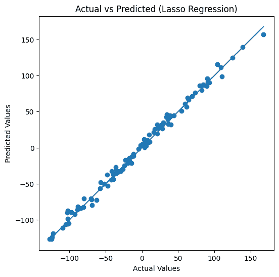
Step 6: Regression Line
- Each point represents one test sample
- X-axis shows actual target values
- Y-axis shows predicted values
- Points closer to a diagonal indicate better predictions
- Spread shows the magnitude of prediction error
- Line shows regression line
y_pred = lasso.predict(X_test)

plt.figure(figsize=(6, 6))
plt.scatter(y_test, y_pred)

min_val = min(y_test.min(), y_pred.min())
max_val = max(y_test.max(), y_pred.max())
plt.plot([min_val, max_val], [min_val, max_val])

plt.xlabel("Actual Values")
plt.ylabel("Predicted Values")
plt.title("Actual vs Predicted (Lasso Regression)")
plt.show()
Output:
Step 7: Plot Lasso Coefficients (Feature Selection)
- Each bar represents one feature’s coefficient
- Zero-height bars indicate discarded features
- Non-zero bars indicate selected important features
- Clearly visualizes Lasso’s feature selection behavior
plt.figure(figsize=(8, 4))
plt.bar(range(len(lasso.coef_)), lasso.coef_, color="green")
plt.xlabel("Feature Index")
plt.ylabel("Coefficient Value")
plt.title("Lasso Regression Coefficients")
plt.show()
Output:
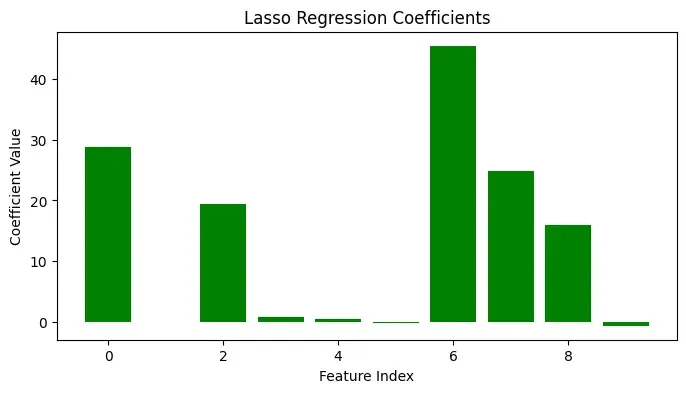
It shows which feature is more important for feature selection.
Step 8: Plot Effect of Regularization Strength (Lasso Path)
- Generates a range of alpha (λ) values on a logarithmic scale
- Trains a new Lasso model for each alpha value
- Stores coefficient values for every feature
- Plots how coefficients change as regularization increases
- Shows that coefficients gradually shrink and drop to zero
- Helps identify stable and important features
alphas = np.logspace(-2, 1, 20)
coefficients = []

for a in alphas:
    model = Lasso(alpha=a)
    model.fit(X_train, y_train)
    coefficients.append(model.coef_)

coefficients = np.array(coefficients)

plt.figure(figsize=(8, 5))
for i in range(coefficients.shape[1]):
    plt.plot(alphas, coefficients[:, i])
plt.xscale("log")
plt.xlabel("Alpha (λ)")
plt.ylabel("Coefficient Value")
plt.title("Lasso Path: Coefficients vs Regularization Strength")
plt.show()
Output:
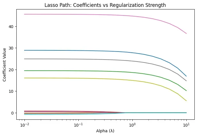
- Each curve represents one feature’s coefficient in the Lasso model
- X-axis shows regularization strength (α) on a logarithmic scale
- As α increases, coefficients shrink toward zero
- Less important features drop to exactly zero
- Important features remain non-zero for longer
- It shows Lasso’s feature selection and overfitting control
Ridge Regression vs Lasso Regression
Let's see the comparison between ridge regression and lasso regression:
| Aspect | Ridge Regression | Lasso Regression |
|---|---|---|
| Regularization | L2 penalty | L1 penalty |
| Feature selection | It does not supports feature selection | It supports feature selection |
| Coefficient shrinkage | Smooth shrinkage | Aggressive shrinkage |
| Zero coefficients | Never | Possible |
| Model sparsity | Dense | Sparse |
| Multicollinearity | Handles very well | Moderate handling |
| Interpretability | Lower | Higher |
Applications
- Feature Selection in ML: Removes irrelevant predictors automatically
- Genomics: Selects influential genes from thousands of variables
- Finance: Identifies key risk factors and predictors
- Text Mining: Chooses important words in high-dimensional text data
- Econometrics: Builds compact explanatory models
Advantages
- Automatic Feature Selection: No extra preprocessing needed
- Sparse Models: Easier interpretation
- Overfitting Reduction: Improves generalization
- High-Dimensional Suitability: Works well when features are many
- Computational Efficiency: Fast optimization methods
Limitations
- Correlated Feature Issue: Selects one feature from a group arbitrarily
- Bias Introduction: Strong regularization may underfit
- Hyperparameter Sensitivity: λ must be tuned carefully
- Limited Group Selection: Not ideal for grouped predictors
- Linear Assumption: Cannot model complex non-linear patterns