Train a model using LightGBM

LightGBM is a tree-based ensemble learning algorithm that uses gradient boosting. Unlike traditional boosting methods, it grows trees leaf-wise (best-first) instead of level-wise.

• Leaf-wise tree growth (better accuracy)
• Histogram-based learning (faster computation)
• Efficient handling of large datasets
• Supports parallel and distributed training

Note: Leaf-wise growth can lead to overfitting, but this is controlled using parameters like max_depth.

Core Techniques Used in LightGBM

1. Histogram-Based Learning

LightGBM converts continuous data into discrete bins, which:

• Reduces memory usage
• Speeds up training
• Avoids repeated sorting

2. Leaf-wise Tree Growth

Instead of splitting all nodes level by level, LightGBM:

• Splits the node with maximum gain
• Builds deeper and more optimized trees

3. Gradient-Based One-Side Sampling (GOSS)

• Keeps data points with large gradients
• Randomly samples from small-gradient data
• Improves training efficiency without much loss in accuracy

4. Exclusive Feature Bundling (EFB)

• Combines sparse features
• Reduces dimensionality
• Improves speed

Implementation to train a model using LightGBM

1. Install and Import Libraries

To train a model using LightGBM we need to install it to our runtime.

!pip install lightgbm

Importing required libraries

import lightgbm as lgb
import numpy as np
import pandas as pd
import matplotlib.pyplot as plt
import seaborn as sns

from sklearn.model_selection import train_test_split, StratifiedKFold
from sklearn.metrics import accuracy_score, precision_score, recall_score, f1_score, classification_report, roc_auc_score
from sklearn.datasets import load_breast_cancer

We import all required Python libraries like NumPy, Pandas, Seaborn, Matplotlib and SKlearn etc.

2. Load Dataset and Preprocessing

The dataset is loaded and split into training and testing sets using stratified sampling to maintain class balance.

data=load_breast_cancer(as_frame=True)
df=data.frame

X=df.drop(columns=["target"])
y=df["target"]

X_train,X_test,y_train,y_test=train_test_split(X,y,test_size=0.2,stratify=y,random_state=42)

3. Exploratory Data Analysis (EDA)

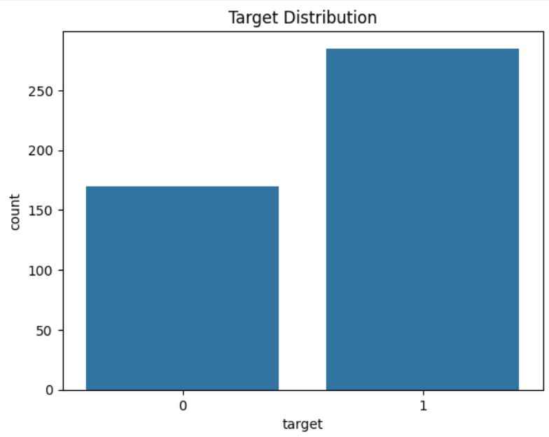
Target Distribution: This plot helps check whether the dataset is balanced or imbalanced.

sns.countplot(x=y_train)
plt.title("Target Distribution")
plt.show()

Output:

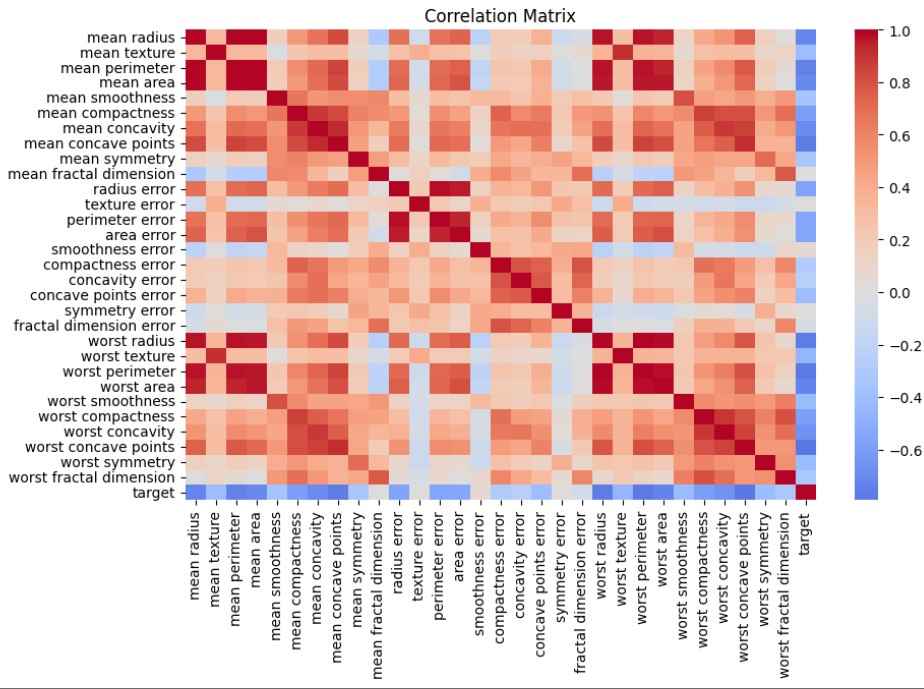
Correlation Matrix: The heatmap shows relationships between features and helps identify highly correlated variables.

corr=df.corr()

plt.figure(figsize=(10,6))
sns.heatmap(corr,cmap="coolwarm",center=0)
plt.title("Correlation Matrix")
plt.show()

Output:

4. Creating LightGBM dataset

LightGBM uses its own optimized dataset format for faster training and better memory usage.

train_data=lgb.Dataset(X_train,label=y_train)
valid_data=lgb.Dataset(X_test,label=y_test,reference=train_data)

5. Define Hyperparameters

These parameters control model learning, complexity, regularization and performance.

params={
"objective":"binary",
"metric":["auc","binary_logloss"],
"boosting_type":"gbdt",
"learning_rate":0.05,
"num_leaves":31,
"max_depth":-1,
"feature_fraction":0.8,
"bagging_fraction":0.8,
"bagging_freq":5,
"lambda_l1":0.1,
"lambda_l2":0.2,
"min_data_in_leaf":20,
"verbose":-1
}

6. Train Model (Latest API)

The model is trained with early stopping to prevent overfitting and logging disabled for cleaner output.

model=lgb.train(
params,
train_data,
num_boost_round=1000,
valid_sets=[train_data,valid_data],
valid_names=["train","valid"],
callbacks=[lgb.early_stopping(50)]
)

Output:

Training until validation scores don't improve for 50 rounds
Early stopping, best iteration is:
[22] train's auc: 0.996956 train's binary_logloss: 0.238247 valid's auc: 0.993056 valid's binary_logloss: 0.257051

7. Predictions

The model outputs probabilities, which are converted into binary predictions using a threshold of 0.5.

y_pred_prob=model.predict(X_test,num_iteration=model.best_iteration)
y_pred=(y_pred_prob>0.5).astype(int)

8. Model Evaluation

These metrics evaluate model performance from different perspectives, especially AUC for classification quality.

accuracy=accuracy_score(y_test,y_pred)
precision=precision_score(y_test,y_pred)
recall=recall_score(y_test,y_pred)
f1=f1_score(y_test,y_pred)
auc=roc_auc_score(y_test,y_pred_prob)

print("Accuracy:",accuracy)
print("Precision:",precision)
print("Recall:",recall)
print("F1 Score:",f1)
print("AUC:",auc)

Output:

Accuracy: 0.9473684210526315
Precision: 0.9583333333333334
Recall: 0.9583333333333334
F1 Score: 0.9583333333333334
AUC: 0.9930555555555556

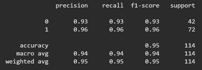
9. Classification Report

Provides a detailed summary of precision, recall and F1-score for each class.

print(classification_report(y_test,y_pred))

Output:

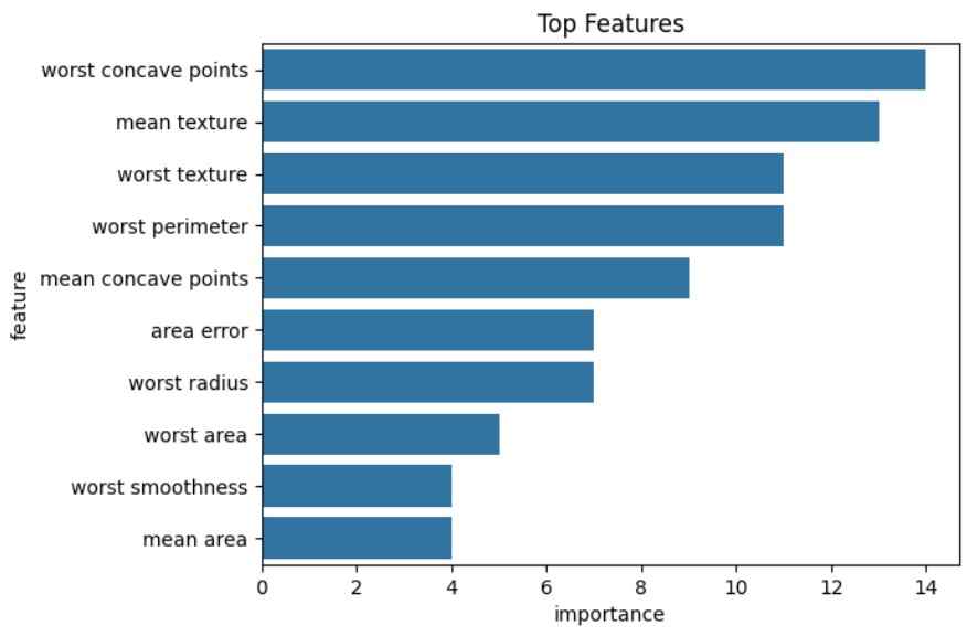
10. Feature Importance

Shows which features contribute most to the model’s predictions.

importance=pd.DataFrame({
"feature":X.columns,
"importance":model.feature_importance()
}).sort_values(by="importance",ascending=False)

sns.barplot(x="importance",y="feature",data=importance.head(10))
plt.title("Top Features")
plt.show()

Output:

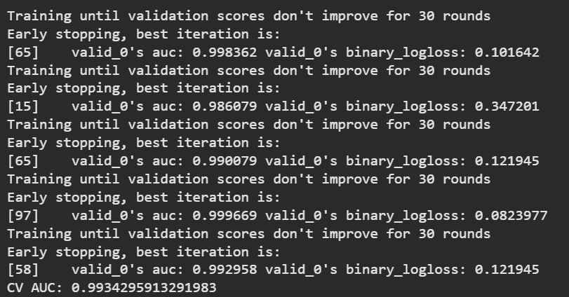
11. Cross-Validation

Cross-validation ensures the model performs well across different data splits (more reliable than a single train-test split).

kf=StratifiedKFold(n_splits=5,shuffle=True,random_state=42)
scores=[]

for train_idx,val_idx in kf.split(X,y):
    X_tr,X_val=X.iloc[train_idx],X.iloc[val_idx]
    y_tr,y_val=y.iloc[train_idx],y.iloc[val_idx]

    train_set=lgb.Dataset(X_tr,label=y_tr)
    val_set=lgb.Dataset(X_val,label=y_val)

    model=lgb.train(
        params,
        train_set,
        num_boost_round=500,
        valid_sets=[val_set],
        callbacks=[
            lgb.early_stopping(30),
            lgb.log_evaluation(0)
        ]
    )

    preds=model.predict(X_val)
    scores.append(roc_auc_score(y_val,preds))

print("CV AUC:",np.mean(scores))

Output:

You can download the source code from here.