Time Series Analysis and Forecasting

To understand how data changes over time, Time Series Analysis and Forecasting are used, which help track past patterns and predict future values. It is widely used in finance, weather, sales and sensor data.

• Focuses on data collected at regular time intervals
• Helps identify trends, seasonality and sudden changes
• Useful for planning, prediction and decision-making
• Common methods include ARIMA, exponential smoothing and machine learning models

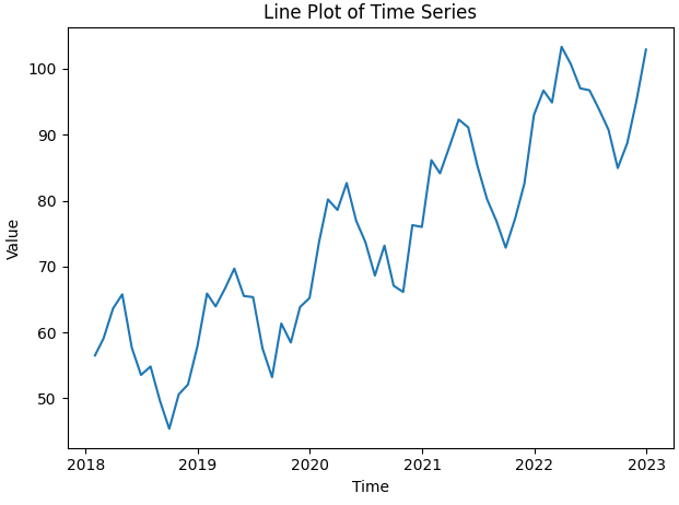
Time series are commonly visualised using a line plot with time on X-axis and observed values on Y-axis. This visualization helps identify trends, fluctuations and underlying patterns.

Importance of Time Series Analysis

• Predicting Future Trends: Helps forecast outcomes like demand, revenue or stock prices.
• Detecting Patterns and Anomalies: Identifies cycles, seasonal effects and unusual behaviors.
• Risk Mitigation: Provides early warnings to prevent potential losses.
• Strategic Planning: Supports budgeting, staffing, inventory and policy decisions.
• Competitive Advantage: Enables faster response and optimized operations.

Components of Time Series Data

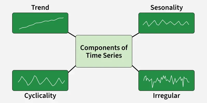
• Trend: Long-term movement of data showing increase, decrease or stability can be linear or nonlinear.
• Seasonality: Regular patterns repeating at fixed intervals like daily, monthly or yearly, often due to seasons or events.
• Cyclical Variations: Long-term fluctuations without fixed periods, linked to economic or business cycles.
• Irregularity (Noise): Random, unpredictable variations caused by events, errors or other unforeseen factors.

When Should You Use Time Series Forecasting

Use Time Series Forecasting When:

• Historical data is consistent and reliable.
• Temporal patterns or trends exist in the data.
• Future behavior depends on past observations.

Avoid Time Series Forecasting When:

• Data is highly noisy or erratic.
• No meaningful historical patterns are present.
• Key influencing factors are unknown or unpredictable.

Types of Time Series

Time series can be grouped based on structure, time interval and statistical behavior. These categories help in selecting the right forecasting method.

1. Univariate vs Multivariate

• Univariate: A univariate time series records only one variable over time, making it simpler to analyze and model.
• Multivariate: A multivariate time series tracks multiple related variables together to show how they influence each other over time.

2. Continuous vs Discrete Time Series

• Continuous: A continuous time series is observed at every moment or at very high frequency like ECG or sensor signals.
• Discrete: A discrete time series is recorded at fixed intervals such as hourly, daily or monthly and is the most common format.

3. Stationary vs Non-Stationary

• Stationary: A stationary series has a constant mean, variance and pattern over time with no trend or seasonality.
• Non-Stationary: A non-stationary series shows changing patterns like trends or seasonality and often needs transformation before modeling.

Preprocessing Time Series Data

Time series preprocessing involves cleaning, transforming and preparing data for analysis or forecasting. The main aim is to improve data quality, remove noise and make the series suitable for modeling. Common tasks include:

• Handling Missing Values: Fill or interpolate missing observations to maintain continuity.
• Dealing with Outliers: Identify and correct extreme values that can distort analysis.
• Stationarity and Transformation: Apply techniques like differencing, detrending or deseasonalizing to stabilize mean and variance over time.
• Scaling and Normalization: Standardize data to improve model performance.
• Variance Stabilization: Apply transformations to reduce variability and improve predictability.

Time Series Preprocessing Techniques

• Stationarity: Keeps mean and variance constant over time.
• Differencing: Removes trends by subtracting previous values.
• Moving Average (MA): Smooths data using a fixed-window average.
• Exponential Moving Average (EMA): Weighted average giving more importance to recent data.
• Missing Value Imputation: Fills gaps using interpolation or statistical methods.
• Outlier Detection and Removal: Identifies and corrects extreme values.
• Scaling: Adjusts value range for comparability.
• Normalization: Standardizes data to a common scale.

Time Series Analysis and Decomposition

Time Series Analysis and Decomposition is used to study sequential data over time, understand patterns and break the series into its core components i.e trend, seasonality and residuals.

Common Techniques:

• Autocorrelation Analysis: Measures correlation between a series and its lagged values to detect patterns.
• Partial Autocorrelation (PACF): Finds direct correlation with lagged values, controlling for intermediate lags.
• Trend Analysis: Identifies long-term direction or movement of the series (linear, exponential or nonlinear).
• Seasonality Analysis: Detects periodic patterns at fixed intervals like daily, weekly or yearly.
• Decomposition: Separates series into trend, seasonal and residual components for easier analysis.
• STL (Seasonal-Trend decomposition using Loess): Decomposes series into seasonal, trend and residual components for modeling.
• Rolling Correlation: Computes correlation between series over a moving window to track changing relationships.

Time Series Visualization

Visualization helps explore, interpret and communicate insights from time-dependent data. Common Visualization Techniques are:

1. Line Plots: Line plots show how a variable changes over time, helping you spot trends, jumps and fluctuations easily.

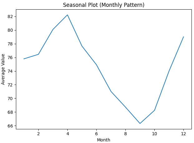
2. Seasonal Plots: Seasonal plots display repeating patterns across months, weeks or seasons to highlight periodic behavior.

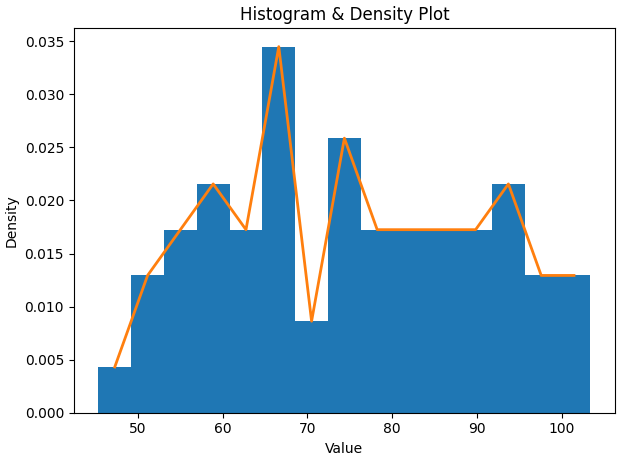
3. Histograms and Density Plots: These plots show the distribution of values in a time series, making it easy to understand common ranges and spread.

4. Autocorrelation and Partial Autocorrelation Plots: ACF and PACF reveal how past values influence current values, helping choose suitable forecasting models.

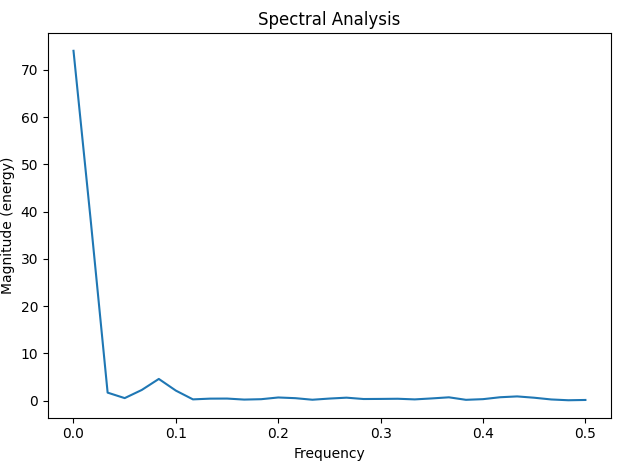
5. Spectral Analysis: Spectral analysis identifies dominant frequency cycles in the data, useful for spotting repeating long-term patterns.

6. Decomposition Plots: Decomposition plots split the series into trend, seasonal and residual parts to clearly show the underlying structure.

Time Series Forecasting Algorithms

Machine Learning Models

• Random Forest: Ensemble model for regression based time series forecasting.
• Gradient Boosting (GBM): Boosted trees to capture complex patterns.
• Generalized Additive Models (GAM): Combines linear and non-linear trends in series.

Deep Learning Models

• RNN: Recurrent networks for sequential dependencies.
• LSTM: Long Short-Term Memory networks handle long-term dependencies.
• GRU: Gated Recurrent Units, a simpler alternative to LSTM.
• Sequence-to-Sequence: Encoder decoder architecture for complex time series.
• CNN-based Models: Capture local temporal patterns using convolutional layers.

Probabilistic and Bayesian Models

• Gaussian Processes: Probabilistic modeling with uncertainty estimation.
• State Space Models: Represent series as latent states evolving over time.
• Dynamic Linear Models (DLM): Time-varying linear models for forecasting.
• Hidden Markov Models (HMM): Models series with underlying hidden states.

Step-By-Step Implementation

Here in this code performs a complete end to end time series forecasting workflow.

Step 1: Install required packages

• Install libraries needed for ARIMA search, decomposition, plotting and evaluation.
• pmdarima provides auto_arima to automatically select ARIMA/SARIMA orders.

!pip install --quiet pmdarima statsmodels matplotlib pandas numpy scikit-learn

Step 2: Importing Libraries

Here we will import numpy, pandas, matplotlib, seaborn, statsmodal and scikit learn.

import numpy as np
import pandas as pd
import matplotlib.pyplot as plt
import seaborn as sns
from statsmodels.tsa.seasonal import seasonal_decompose
from statsmodels.tsa.stattools import adfuller
from sklearn.metrics import mean_absolute_error, mean_squared_error
import pmdarima as pm

Step 3: Generate synthetic monthly time series

• Create a monthly date index for periods points.
• Build a linear trend component and a yearly seasonal component.
• Add Gaussian noise to make the series realistic.

periods = 120
time_index = pd.date_range("2015-01-01", periods=periods, freq="M")
trend = np.linspace(50, 120, periods)
season = 10 * np.sin(2 * np.pi * time_index.month / 12)
noise = np.random.normal(0, 5, periods)

ts = trend + season + noise

Step 4: Create DataFrame

• Put the generated series into a pandas DataFrame with a Date index.
• Setting the Date as index is important for plotting, resampling and time aware operations.

data = pd.DataFrame({"Date": time_index, "Value": ts})
data.set_index("Date", inplace=True)
data.head()

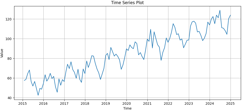
Step 5: Visualize the raw time series

• Plot the observed series to inspect trend and seasonality.
• A quick visual check helps decide preprocessing and modelling choices.

plt.figure(figsize=(12,5))
plt.plot(data.Value)
plt.title("Time Series Plot")
plt.xlabel("Time")
plt.ylabel("Value")
plt.grid(True)
plt.show()

Output:

Step 6: Handle missing values

• Interpolate missing values if present keeps continuity for time series algorithms.
• This step is safe for most continuous series and simple synthetic data.

data.Value = data.Value.interpolate()

Step 7: Outlier detection and cleaning (z-score method)

• Compute z-scores to identify extreme values relative to mean/std.
• Replace values with z-score > 3 by the series median.

z = np.abs((data.Value - data.Value.mean()) / data.Value.std())
data["Value_clean"] = np.where(z > 3, data.Value.median(), data.Value)

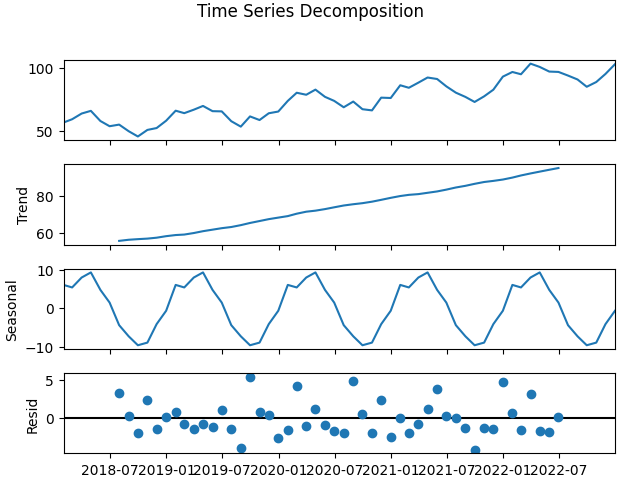
Step 8: Time series decomposition

• Use seasonal_decompose (additive model, period=12 for monthly seasonality).
• Visualize trend, seasonal component and residuals to inform modelling choice.
• Decomposition helps decide additive vs multiplicative models.

decomp = seasonal_decompose(data.Value_clean.dropna(), model="additive", period=12)
decomp.plot()
plt.show()

Output:

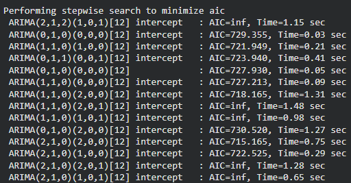
Step 9: Train automatic SARIMA

• Use pmdarima.auto_arima to search for best seasonal ARIMA parameters automatically.
• seasonal=True and m=12 set monthly seasonality.

model = pm.auto_arima(
    train,
    seasonal=True,
    m=12,
    trace=True,
    error_action="ignore",
    suppress_warnings=True
)

model.summary()

Output:

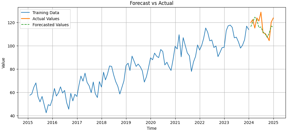
Step 10: Forecast on test set and plot results

• Forecast the next 12 periods and align predictions with test index.
• Plot training data, actual test values and forecasted values for visual comparison.

forecast = model.predict(n_periods=12)
forecast = pd.Series(forecast, index=test.index)

plt.figure(figsize=(12,5))
plt.plot(train, label='Training Data')
plt.plot(test, label='Actual Values', linewidth=2)
plt.plot(forecast, label='Forecasted Values', linestyle="--")
plt.title("Forecast vs Actual")
plt.xlabel("Time")
plt.ylabel("Value")
plt.legend()
plt.grid(True)
plt.show()

Output:

You can download full code form here.

Applications

Time series forecasting is widely used across industries to predict future values and support decision making:

• Weather and Climate Modeling: Predict temperature, rainfall and extreme events.
• Finance and Stock Prediction: Predict stock prices, returns and market trends.
• Demand Forecasting: Estimate product or service demand to optimize inventory.
• Retail Sales: Predict sales patterns and seasonal trends.
• Traffic Forecasting: Estimate traffic flow for urban planning and route optimization.

Limitations

Time series forecasting is a useful technique but comes with several limitations and challenges:

• Missing Values: Gaps in data reduce accuracy and model reliability.
• Limited Data: Short historical records hinder accurate forecasting.
• Non-Stationarity: Changing mean or variance over time affects model stability.
• Seasonal Drift: Seasonal patterns may shift over years, complicating predictions.
• Concept Drift: Underlying patterns evolve over time, reducing model relevance.
• Overfitting in ML/DL Models: Complex models may capture noise instead of true patterns, harming generalization.