Steps to Build a Machine Learning Model

Machine Learning is a field of Artificial Intelligence that enables computers to learn from data and make decisions without being explicitly programmed. By identifying hidden patterns and relationships within data, ML models can generalize and make predictions on unseen data.

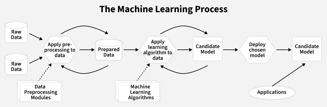
Machine learning models helps us extract meaningful patterns, trends and insights from vast amounts of data, enabling better decisions and intelligent automated systems.

Why Machine Learning is Important

• Automation: Eliminates manual and repetitive tasks using intelligent systems.
• Prediction and Forecasting: Enables accurate decision-making through data-driven predictions.
• Real time Insights: Detects patterns instantly for use cases like fraud detection.
• Personalization: Delivers user-specific recommendations by learning individual preferences.
• Efficiency and Optimization: Enhances performance, reduces errors and lowers operational costs.

How to Build a Machine Learning Model

1. Define the Problem

Clearly understand what the model is supposed to predict or classify, ensuring the ML task matches the actual objective.

• Identify the business goal or research purpose behind building the model.
• Decide whether the task is regression, classification, clustering or forecasting.
• Determine the type of data required and the expected output format.

2. Collect Data

Collect all relevant and high quality data from reliable sources, as the dataset forms the foundation of any machine learning model.

• Gather data from databases, sensors, surveys, web APIs or public datasets like Kaggle and UCI.
• Ensure the dataset is large, clean and representative of the real problem.
• Combine data from multiple sources if needed to improve coverage and diversity.
• Check early for issues like missing values, noise and imbalance to avoid problems later.

3. Data Cleaning and Preprocessing

Prepare the raw data for modeling by fixing errors, handling missing values and transforming it into a clean and usable form.

• Remove duplicates and correct inconsistent or incorrect entries.
• Handle missing values using imputation, deletion or interpolation techniques.
• Normalize or scale numerical features for stable and faster model training.
• Encode categorical variables using Label Encoding, One-Hot Encoding or Target Encoding.

4. Exploratory Data Analysis (EDA)

Analyze the dataset to understand patterns, distributions and relationships between features before building the model.

• Visualize data using graphs, charts, heatmaps and pair plots.
• Check statistical summaries to understand mean, variance, skewness and outliers.
• Study feature relationships and correlations to identify useful predictors.
• Detect anomalies, trends and hidden patterns that influence model design.

5. Feature Selection and Engineering

Select the most relevant features and create new meaningful ones to enhance model accuracy, reduce complexity and improve learning.

• Remove irrelevant, redundant or noisy features that harm performance.
• Use techniques like Correlation Analysis, Chi-square, ANOVA, PCA, Mutual Information.
• Good feature engineering often improves performance more than switching algorithms.

6. Split Data into Training and Testing Sets

Divide the dataset so the model learns from one part and is evaluated fairly on unseen data.

• Ensures the model is evaluated on unseen data, preventing overfitting.
• Stratified splits are used for classification to maintain class balance.
• Optionally create a validation set or use cross validation for better tuning.

7. Select a Machine Learning Algorithm

Choose the most suitable algorithm based on the problem type, data characteristics, and performance requirements.

• Pick algorithms depending on the task like Linear Regression, Random Forest, SVM, KNN, Neural Networks.
• Consider factors like speed, accuracy, interpretability, scalability and dataset size.
• For smaller datasets, simpler models often perform better large datasets may benefit from deep learning.

8. Train the Model

Train the selected algorithm on the prepared training data so it can learn patterns, relationships and decision boundaries

• Adjust model parameters iteratively to minimize loss.
• Monitor learning curves to track training progress and detect issues early.
• Ensure the model converges properly and is not overfitting or diverging.

9. Evaluate Model Performance

Test the trained model on unseen data to measure how well it generalizes and how reliable its predictions are.

• Use metrics like Accuracy, Precision, Recall, F1-score, RMSE, MAE, R² depending on task type.
• Compare training vs testing results to detect overfitting or underfitting.
• Use confusion matrices, ROC curves and error analysis for deeper evaluation.

10. Hyperparameter Tuning

Optimize the model’s hyperparameters to achieve higher accuracy, stability and better generalization.

• Use Grid Search, Random Search, Bayesian Optimization or cross-validation techniques.
• Adjust settings like learning rate, depth, number of trees, batch size, etc.
• Aim to balance model complexity vs performance to avoid overfitting.

11. Deploy the Model

Make the trained model available for real-world use by integrating it into applications, systems or services.

• Deploy on cloud platforms or mobile systems.
• Set up APIs, model servers or pipelines using Flask, FastAPI, TensorFlow Serving or Docker.
• Monitor model performance in production to detect drift or degradation.

12. Monitor and Maintain the Model

Continuously track the model’s performance in production and update it when real-world data or patterns start to change.

• Retrain the model with new or updated data whenever accuracy declines.
• Detect data drift, concept drift or model degradation using monitoring tools.
• Log predictions, errors and feedback to identify issues early.
• Regular maintenance ensures the model remains reliable, accurate and relevant over time.

Common Terms Used in Machine Learning

1. Features: Input variables or attributes used by the model to make predictions can be numerical, categorical or derived through feature engineering.
2. Labels: The target variable that the model tries to predict during supervised learning.
3. Training Set: Dataset used to teach the model patterns and relationships between features and labels.
4. Validation Set: A separate dataset used for tuning hyperparameters and preventing overfitting during model development.
5. Test Set: Final dataset used to check how well the trained model generalizes to unseen data.
6. Overfitting: A condition where the model memorizes training data but fails on new data hence solved using regularization, dropout and cross-validation.
7. Underfitting: Occurs when the model is too simple to learn underlying patterns, resulting in poor performance on both training and test data.
8. EDA (Exploratory Data Analysis): Process of visualizing, summarizing and understanding data distributions, outliers and relationships before modeling.
9. Hyperparameters: Model settings defined before training like learning rate, number of trees, batch size, etc that significantly affect model performance.
10. Cross-Validation: Technique to evaluate model performance by splitting data into multiple folds, ensuring stable and reliable accuracy.
11. Feature Engineering: Process of creating, transforming or selecting meaningful features to improve model learning and accuracy.
12. Model Deployment: Making a trained model usable in real applications through APIs, cloud platforms or integration into software systems.

Step-By-Step Implementation

Here we implemented a complete end to end Machine Learning workflow to predict customer churn using Telecom dataset.

Step 1: Import Required Libraries

• import Pandas and NumPy for data handling and numerical computations.
• import Matplotlib is used for visual analysis.
• associations() is used for categorical correlation.

import pandas as pd
import numpy as np
import matplotlib.pyplot as plt
from dython.nominal import associations

Step 2: Load the Dataset

• Load the CSV file into a dataframe.
• Check dataset summary, missing values and target distribution.

df = pd.read_csv('WA_Fn-UseC_-Telco-Customer-Churn.csv')

df.head()  
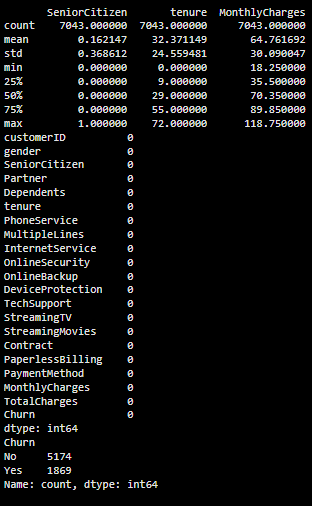
print(df.describe())
print(df.isnull().sum())
print(df['Churn'].value_counts())

Output:

Step 3: Data Cleaning & Feature Engineering

• Convert invalid values in TotalCharges and convert to numeric.
• Convert SeniorCitizen to string.
• Create binary target label ChurnTarget.

df['TotalCharges'] = df['TotalCharges'].replace('', np.nan)
df['TotalCharges'] = pd.to_numeric(df['TotalCharges'], errors='coerce').fillna(0)

df['SeniorCitizen'] = df['SeniorCitizen'].astype(str)

df['ChurnTarget'] = df['Churn'].apply(lambda x: 1 if x=='Yes' else 0)

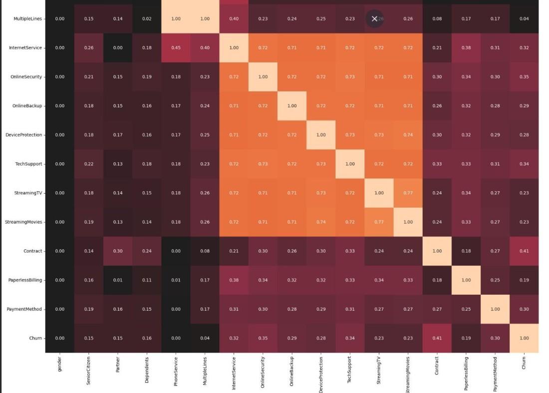
Step 4: Feature Selection Using Correlation

• Separate numeric and categorical features.
• Select features with correlation > 0.3
• Combine selected features into one list.

target = 'ChurnTarget'
num_features = df.select_dtypes(include=[np.number]).columns.drop(target)
correlations = df[num_features].corrwith(df[target])
selected_num_features = correlations[abs(correlations) > 0.3].index.tolist()

cat_features = df.drop('customerID', axis=1).select_dtypes(include='object').columns
assoc = associations(df[cat_features], nominal_columns='all', plot=False)
corr_matrix = assoc['corr']

selected_cat_features = corr_matrix[corr_matrix.loc['Churn'] > 0.3].index.tolist()
selected_cat_features = selected_cat_features[:-1]

print("Selected Numeric Features:", selected_num_features)
print("Selected Categorical Features:", selected_cat_features)

selected_features = selected_num_features + selected_cat_features

Output:

Step 5: Train-Validation-Test Split

• Use selected features as predictors X and churn target as y.
• Split data into 60% train, 20% validation, 20% test with stratification.

from sklearn.model_selection import train_test_split

X = df[selected_features]
y = df[target]

cat_features = X.select_dtypes(include=['object']).columns.tolist()
num_features = X.select_dtypes(include=['number']).columns.tolist()

X_train_val, X_test, y_train_val, y_test = train_test_split(X, y, test_size=0.2,
                                                            random_state=42, stratify=y)

X_train, X_val, y_train, y_val = train_test_split(X_train_val, y_train_val,
                                                  test_size=0.25, random_state=42,
                                                  stratify=y_train_val)

Step 6: Build ML Pipeline & Train Logistic Regression

• One hot encode categorical variables.
• Use pipeline for easy model transformation and training.

from sklearn.compose import ColumnTransformer
from sklearn.pipeline import Pipeline
from sklearn.preprocessing import OneHotEncoder
from sklearn.linear_model import LogisticRegression
from sklearn.metrics import classification_report

preprocessor = ColumnTransformer(
    transformers=[
        ('num', 'passthrough', num_features),
        ('cat', OneHotEncoder(handle_unknown='ignore'), cat_features)
    ])

pipeline = Pipeline(steps=[
    ('preprocessor', preprocessor),
    ('classifier', LogisticRegression(max_iter=1000))
])

pipeline.fit(X_train, y_train)

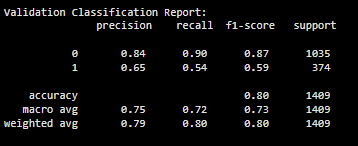
y_val_pred = pipeline.predict(X_val)
print("Validation Classification Report:\n", classification_report(y_val, y_val_pred))

Output:

Step 7: Hyperparameter Tuning Using GridSearchCV

• Tune model parameters using recall metric.
• Select best settings based on validation performance.

from sklearn.model_selection import GridSearchCV

param_grid = {
    'classifier__C': [0.1, 1, 10, 100],
    'classifier__solver': ['lbfgs', 'liblinear']
}

grid_search = GridSearchCV(pipeline, param_grid, cv=5, scoring='recall')
grid_search.fit(X_train, y_train)

print("Best Hyperparameters:", grid_search.best_params_)

y_test_pred = grid_search.predict(X_test)
print("Test Classification Report:\n", classification_report(y_test, y_test_pred))

Step 8: Compare Performance with Multiple ML Models

• Train different ML models like decision tree, random forest, support vetor machine, etc on same pipeline.
• Calculate recall on test set.
• Store results and visualize comparison.

from sklearn.tree import DecisionTreeClassifier
from sklearn.ensemble import RandomForestClassifier, GradientBoostingClassifier
from sklearn.svm import SVC
from xgboost import XGBClassifier
from lightgbm import LGBMClassifier
from sklearn.metrics import recall_score

models = {
    'Logistic Regression': LogisticRegression(max_iter=1000),
    'Decision Tree': DecisionTreeClassifier(),
    'Random Forest': RandomForestClassifier(),
    'SVM': SVC(),
    'Gradient Boosting': GradientBoostingClassifier(),
    'XGBoost': XGBClassifier(use_label_encoder=False, eval_metric='logloss'),
    'LightGBM': LGBMClassifier()
}

results = []

for name, model in models.items():
    pipe = Pipeline(steps=[
        ('preprocessor', preprocessor),
        ('classifier', model)
    ])
    pipe.fit(X_train, y_train)
    y_pred = pipe.predict(X_test)
    recall = recall_score(y_test, y_pred)
    
    results.append((name, recall))

results

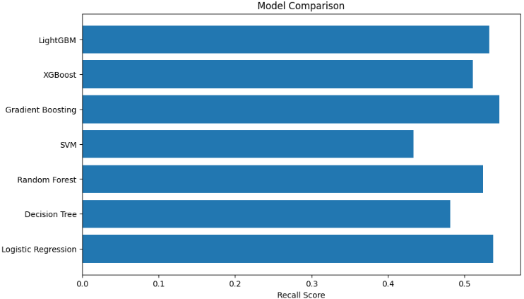
Step 9: Plot Recall Comparison

• Visualize recall score performance for each model.
• Helps choose best performing ML model.

model_names = [r[0] for r in results]
test_recalls = [r[1] for r in results]

plt.figure(figsize=(10, 6))
plt.barh(model_names, test_recalls)
plt.xlabel('Recall Score')
plt.title('Model Comparison')
plt.show()

Output:

Step 10: Save Best Model

Save logistic regression model with best parameters Used later for deployment (FastAPI, Streamlit etc.)

import joblib

best_model = grid_search.best_estimator_
joblib.dump(best_model, 'model.joblib')

You can download full code from here

Model Deployment Methods

• REST API (FastAPI / Flask): Expose model predictions through API endpoints for integration with applications.
• Streamlit / Gradio: Build interactive web UIs for testing and showcasing machine learning models.
• Docker Containers: Package the entire model environment for consistent and portable deployment.
• Cloud Platforms: Host, scale and manage ML models using cloud services and serverless deployments.

Applications

• Healthcare: Used for disease prediction, medical image analysis and personalized treatment.
• Finance: Helps in fraud detection, credit scoring and algorithmic trading.
• E-commerce: Powers recommendation systems, demand forecasting and customer behavior analysis.
• Telecom: Enables customer churn prediction, network optimization, and fault detection.
• Autonomous Systems: Drives self-driving cars, drones and intelligent robotics.

Limitation

• Data quality issues: Poor, noisy or missing data reduces model accuracy and reliability.
• Imbalanced datasets: Unequal class distribution causes biased predictions toward majority classes.
• Model overfitting and underfitting: Overfitting memorizes data, while underfitting fails to learn patterns.
• Computational cost and scalability: Large datasets and complex models demand high processing power and memory.
• Interpretability and explainability: Complex models are hard to understand, making decisions less transparent.