Recovering Feature Names of explained_variance_ratio_ in PCA with sklearn

Principal Component Analysis (PCA) is a powerful technique used in data science for dimensionality reduction, feature extraction, and data visualization. One of the key outputs of PCA is the explained_variance_ratio_, which indicates the proportion of the dataset's variance that each principal component accounts for. However, understanding which original features contribute to these principal components can be crucial for interpreting the results. This article will guide you through the process of recovering feature names associated with the explained_variance_ratio_ in PCA using Scikit-Learn.

Introduction to Principal Component Analysis

PCA is an unsupervised learning algorithm that transforms the original features into a new set of features called principal components. These components are orthogonal to each other and are ordered by the amount of variance they explain in the data. The primary goals of PCA include:

• Dimensionality Reduction: Reducing the number of features while retaining most of the variance.
• Feature Extraction: Identifying new features that capture the essential information.
• Data Visualization: Simplifying the visualization of high-dimensional data.

Understanding Explained Variance Ratio

Explained variance ratio is a measure of the percentage of the total variance in a given dataset for each principal component. The explained variance ratio of a principal component is measured as the ratio of its eigenvalue to the sum of the eigenvalues of all the principal components.

Using the explained_variance_ratio attribute (from Sklearn PCA), one can access the explained variance ratio for each principal component. The code is as follows:

The steps for the above code as follows:

• Create synthetic classification data with 10 features.
• Apply PCA with n_components as 5.
• Access the explained variance ratio using the explained_variance_ratio attribute from Sklearn PCA.
• Print the explained variance ratio for each principal component.

from sklearn.decomposition import PCA
from sklearn.datasets import make_classification
import numpy as np

# create a synthetic classificatiom dataset with 10 features
X, y = make_classification(n_samples=1000, 
                           n_features=10, 
                           random_state=42)

# Feature names
feature_names = [f"Feature {i+1}" for i in range(X.shape[1])]

# Applying PCA
pca = PCA(n_components=5)
X_pca = pca.fit_transform(X)

# access explained variance ratio for each principal component
explained_variance_ratio = pca.explained_variance_ratio_
for indx, evr in enumerate(explained_variance_ratio):
    print(f"PC{indx+1}: {evr:.2f}")

Output:

PC1: 0.31 
PC2: 0.15 
PC3: 0.11 
PC4: 0.09 
PC5: 0.09

Visualization Plot for Explained Variance Ratio

Let's create a visualisation plot for explained variance ratio for each principal component.

import matplotlib.pyplot as plt

fig, ax = plt.subplots()
# set x and y values
x = np.arange(1, len(explained_variance_ratio) + 1)
y = explained_variance_ratio
# plot
ax.plot(x, y, marker='o')
# set label and title
ax.set_xlabel('Principal Component')
ax.set_ylabel('Explained Variance Ratio')
ax.set_title('Explained Variance Ratio by Principal Component')
plt.show()

Output:

The above code plots the chart of variance proportions for each principal components. This is useful especially when trying to identify how much variation is explained by each of the principal components as well as when seeking to visualize the components within the data samples.

Recovering Feature Names in PCA

PCA is an orthogonal linear transformation that transforms the data into a new coordinate system. So, the features retrieved from PCA are not the original features. Information about the original feature is available in the pca attribute: components. To understand which original features contribute to the principal components, we need to examine the pca.components_ attribute.

Let's follow the below steps to recover feature names.

Step 1: Retraining and Applying PCA

First of all, to balance them, you need to fit a PCA model to your data.

from sklearn.decomposition import PCA
import numpy as np

# Example data
X = np.array([[1, 2, 3], [4, 5, 6], [7, 8, 9]])

# Example feature names
feature_names = ["Feature1", "Feature2", "Feature3"]

# Fitting PCA
pca = PCA(n_components=2)
X_pca = pca.fit_transform(X)

Step 2: Access Component Weights

After applying PCA to the given data and finding the values of the first few principal components, it is possible to get the component weights which give the information about contribution of each original feature to the principal components.

# Accessing the component weights
component_weights = pca.components_
print("Component Weights:\n", component_weights)

Output:

Component Weights:  
[[ 0.57735027  0.57735027  0.57735027] 
 [-0.81649658  0.40824829  0.40824829]]

Step 3: Create Mapping Between Feature Names and Component Weights

Construct a list where each element is a mapping of the initial feature name and its corresponding weight for each of the principal components.

# Create a mapping between component weights and feature names
feature_weights_mapping = {}
for i, component in enumerate(component_weights):
    component_feature_weights = zip(feature_names, component)
    feature_weights_mapping[f"Component {i+1}"] = sorted(
      component_feature_weights, key=lambda x: abs(x[1]), reverse=True)

Step 4: Display Feature Contributions

They should show the name of each feature and its corresponding weight meaning how much it contributes to each of the principal component.

# Accessing feature names contributing to Component 1
print("Feature names contributing to Component 1:")
for feature, weight in feature_weights_mapping["Component 1"]:
    print(f"{feature}: {weight}")

# Accessing feature names contributing to Component 2
print("Feature names contributing to Component 2:")
for feature, weight in feature_weights_mapping["Component 2"]:
    print(f"{feature}: {weight}")

Output:

Feature names contributing to Component 1: 
Feature1: 0.577350269189626 
Feature2: 0.5773502691896255 
Feature3: 0.5773502691896255 
Feature names contributing to Component 2: 
Feature1: -0.8164965809277258 
Feature2: 0.40824829046386313 
Feature3: 0.40824829046386313

Example: Recovering Feature Names After PCA with Scikit-Learn

Here's an example code snippet demonstrating how to recover feature names after performing PCA using scikit-learn. Here we make use of iris dataset. It consists of 3 different types of irises (Setosa, Versicolour, and Virginica) and has 4 features: sepal length, sepal width, petal length, and petal width. The code is as follows:

from sklearn import datasets
from sklearn.decomposition import PCA
# load iris dataset
iris = datasets.load_iris()
# features
feature_names = iris.feature_names

# Specify the number of components you want
pca_iris = PCA(n_components=3)
X_pca = pca_iris.fit_transform(iris.data)
component_weights = pca_iris.components_

# Create a mapping between component weights and feature names
feature_weights_mapping = {}
for i, component in enumerate(component_weights):
  component_feature_weights = zip(feature_names, component)
  sorted_feature_weight = sorted(
      component_feature_weights, key=lambda x: abs(x[1]), reverse=True)
  feature_weights_mapping[f"Component {i+1}"] = sorted_feature_weight
  
# Accessing feature names contributing to Principal Component
print("Feature names contributing to Principal Components")
for feature, weight in feature_weights_mapping.items():
  print(f"{feature}: {weight}") 

Output:

Feature names contributing to Principal Components: 
Component 1: [('petal length (cm)', 0.8566706059498349), ('sepal length (cm)', 0.36138659178536864), ('petal width (cm)', 0.3582891971515507), ('sepal width (cm)', -0.08452251406456868)] 
Component 2: [('sepal width (cm)', 0.7301614347850266), ('sepal length (cm)', 0.6565887712868423), ('petal length (cm)', -0.17337266279585706), ('petal width (cm)', -0.07548101991746337)] 
Component 3: [('sepal width (cm)', 0.5979108301000855), ('sepal length (cm)', -0.5820298513060651), ('petal width (cm)', 0.5458314320200757), ('petal length (cm)', 0.0762360758209632)]

In the above code, n_components is set to 3. Hence, PCA will create 3 new features that are a linear combination of the 4 original features. Following the PCA data analysis and fitting the model, the next step is to get hold of the component weights by using the command: pca.components_. Finally, for each principal components, we generate the mapping that assigns names to the matrix columns and weights to the features. Last for all, we want to know the features associated to the principal components so we print them out.

Visualizing - Explained Variance ratio and Cumulative Explained Variance Ratio

Let's plot the explained variance ratio and cumulative explained variance for each principal component.

import numpy as np
import matplotlib.pyplot as plt
# explained variance ratio
explained_variance_ratio = pca_iris.explained_variance_ratio_
cum_evr = np.cumsum(explained_variance_ratio)
# plot 
plt.figure(figsize=(8, 6))
# plot explained variance ratio
plt.bar(range(1, len(explained_variance_ratio) + 1), 
        explained_variance_ratio, alpha=0.7, align='center', 
        label='Individual explained variance')
# plot cumulative explained variance ratio
plt.step(range(1, len(explained_variance_ratio) + 1), 
         cum_evr, where='mid', 
         label='Cumulative explained variance')
plt.xlabel('Principal components')
plt.ylabel('Explained variance ratio')
plt.legend(loc='best')
plt.title('Explained Variance Ratio vs Principal Components')
plt.show()

Output:

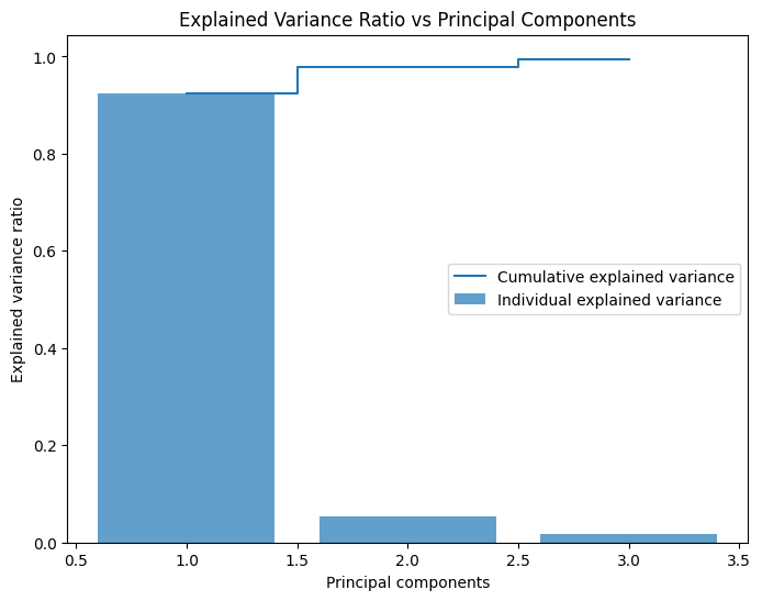
Here we get the explained variance ratio from the pca object using the explained_variance_ratio attribute and calculate the cumulative sum of the explained variance ratio using the cumsum() method provided by Numpy. Finally, we plot the explained variance ratio and cumulative explained variance ratio for each principal component using Matplotlib.

Practical Applications

Understanding the feature contributions to principal components can be useful in various scenarios:

• Feature Selection: Identifying the most important features for model building.
• Data Interpretation: Gaining insights into the underlying structure of the data.
• Dimensionality Reduction: Reducing the number of features while retaining essential information.

Conclusion

Recovering the feature names associated with the explained_variance_ratio_ in PCA is a crucial step in interpreting the results of PCA. By examining the pca.components_ attribute, we can understand the contribution of each original feature to the principal components. This process enhances our ability to make informed decisions based on the PCA results.