Independent Component Analysis - ML

Independent Component Analysis (ICA) is a technique used to separate mixed signals into their independent, non-Gaussian components. Its aim is to find a linear transformation of data that maximizes statistical independence among the components. ICA is widely used in audio & image processing and biomedical signal analysis to isolate distinct sources from mixed signals.

Statistical Independence Concept

Statistical independence refers to the idea that two random variables: X and Y are independent if knowing one does not affect the probability of the other. Mathematically, this means the joint probability of X and Y is equal to the product of their individual probabilities.

P(X \cap Y) = P(X) \cdot P(Y) or P(X \cap Y) = P(X) \cdot P(Y)

Assumptions in ICA

ICA operates under two key assumptions:

1. The source signals are statistically independent of each other.
2. The source signals have non-Gaussian distributions.

These assumptions allow ICA to effectively separate mixed signals into independent components, a task that traditional methods like PCA cannot achieve

Mathematical Representation of ICA

The observed random vector is X= (x_1 , \dots , x_m )^T representing the observed data with m components. The hidden components are represented by the random vector S = (s_{1} ,\dots, s_{n})^T where n is the number of hidden sources.

The observed data X is transformed into hidden components S using a linear static transformation representation by the matrix W.

S = WX

The goal is to transform the observed data X in a way that the resulting hidden components are independent. The independence is measured by some function F(s_1 , \dots, s_n). The task is to find the optimal transformation matrix W that maximizes the independence of hidden components.

Cocktail Party Problem in ICA

To better understand how Independent Component Analysis (ICA) works let’s look at a classic example known as the Cocktail Party Problem

Here there is a party going into a room full of people.

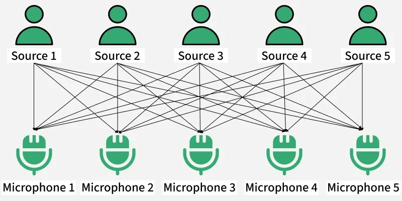
• There is 'n' number of speakers in that room and they are speaking simultaneously at the party.
• In the same room, there are also 'n' microphones placed at different distances from the speakers which are recording 'n' speakers' voice signals.

Hence the number of speakers is equal to the number of microphones in the room. Now using these microphones' recordings, we want to separate all the 'n' speakers voice signals in the room given that each microphone recorded the voice signals coming from each speaker of different intensity due to the difference in distances between them.

Decomposing the mixed signal of each microphone's recording into an independent source's speech signal can be done by using the machine learning technique independent component analysis.

\begin{bmatrix}y_1 \\y_2 \\\vdots \\y_n\end{bmatrix}=\mathbf{W}\begin{bmatrix}x_1 \\x_2 \\\vdots \\x_n\end{bmatrix}

where X_1, X_2, \dots, X_n are the original signals present in the mixed signal and Y_1, Y_2, \dots, Y_n are the new features and are independent components that are independent of each other.

Implementing ICA in Python

Step 1: Import necessary libraries

First we will import numpy, sklearn, FastICA and matplotlib.

import numpy as np
from sklearn.decomposition import FastICA
import matplotlib.pyplot as plt

Step 2: Generate Random Data and Mix the Signals

In this step we create three separate signals: a sine wave, a square wave and random noise. These represent different types of real-world signals. We use NumPy to generate 200 time points between 0 and 8.

• signal_1: A sine wave like a tuning fork tone.
• signal_2: A square wave like a digital signal (on/off).
• signal_3: A random noise signal using the Laplace distribution which has sharper peaks than normal distribution.
• np.c_[]: Combine all three 1D signals into a single 2D array.
• 0.2 is the standard deviation of the noise

np.random.seed(42)
samples = 200
time = np.linspace(0, 8, samples)

signal_1 = np.sin(2 * time)
signal_2 = np.sign(np.sin(3 * time))
signal_3 = np.random.laplace(size=samples)

S = np.c_[signal_1, signal_2, signal_3]
S += 0.2 * np.random.normal(size=S.shape)

A = np.array([[1, 1, 1], [0.5, 2, 1], [1.5, 1, 2]])
X = S.dot(A.T) 

Step 3: Apply ICA to unmix the signals

In this step we apply Independent Component Analysis using the FastICA class from Scikit-learn. We first create an instance of FastICA and set the number of independent components to 3 matching the number of original signals.

ica = FastICA(n_components=3)
S_ = ica.fit_transform(X)

Step 4: Visualize the signals

In this step we use Matplotlib to plot and compare the original sources, mixed signals and the signals recovered using ICA.

We create three subplots:

• First shows the original synthetic signals
• Second displays the observed mixed signals
• Third shows the estimated independent sources obtained from ICA

plt.figure(figsize=(8, 6))

plt.subplot(3, 1, 1)
plt.title('Original Sources')
plt.plot(S)

plt.subplot(3, 1, 2)
plt.title('Observed Signals')
plt.plot(X)

plt.subplot(3, 1, 3)
plt.title('Estimated Sources (FastICA)')
plt.plot(S_)

plt.tight_layout()
plt.show()

Output:

Difference between PCA and ICA

Advantages

• Separates mixed signals into independent components, useful in signal and image processing.
• Non-parametric, so it doesn’t assume a specific data distribution.
• Works without labeled data as an unsupervised technique.
• Helps in feature extraction by identifying important data patterns.

Disadvantages

• Assumes non-Gaussian sources, so it may fail if data is Gaussian.
• Assumes linear mixing, making it less effective for nonlinear data.
• Can be computationally expensive for large datasets.

Related Article:

• Blind source separation using FastICA in Scikit Learn