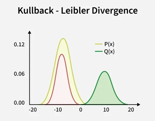
Kullback Leibler (KL) Divergence

Kullback Leibler Divergence is a measure from information theory that quantifies the difference between two probability distributions.

1. It tells us how much information is lost when we approximate a true distribution P with another distribution Q.
2. KL divergence is also called relative entropy and is non negative and asymmetric D_{\mathrm{KL}}(P \parallel Q) \neq D_{\mathrm{KL}}(Q \parallel P) .
3. It measures the extra number of bits needed to encode data from P if we use a code optimized for Q instead of the true distribution P.

Mathematical Implementation

Mathematical Implementation of KL Divergence for discrete and continuous distributions:

1. Discrete Distributions:

For two discrete probability distributions P = {p₁, p₂, ..., p_n} and {q₁, q₂, ...., q_n} over the same set:

D_{\mathrm{KL}}(P \parallel Q) = \sum_{i=1}^{n} p_i \log \frac{p_i}{q_i}

Step by step:

• For each outcome i, compute p_i log(p_i / q_i).
• Sum all these terms to get the total KL divergence.

2. Continuous Distributions:

For continuous probability density functions p(x) and q(x):

D_{\mathrm{KL}}(P \parallel Q) = \int p(x) \log \frac{p(x)}{q(x)} \, dx

• Integration replaces summation for continuous variables.
• Gives the expected extra information in nats or bits required when assuming q(x) instead of p(x).

Properties

Properties of KL Divergence are:

1. Non Negativity: KL divergence is always non negative and equals zero if and only if P=Q almost everywhere.

D_{\mathrm{KL}}(P \parallel Q) \ge 0

2. Asymmetry: KL divergence is not symmetric so it is not a true distance metric.

D_{\mathrm{KL}}(P \parallel Q) \neq D_{\mathrm{KL}}(Q \parallel P)

3. Additivity for Independent Distributions: If X and Y are independent:

D_{\mathrm{KL}}(P_{X,Y} \parallel Q_{X,Y}) = D_{\mathrm{KL}}(P_X \parallel Q_X) + D_{\mathrm{KL}}(P_Y \parallel Q_Y)

4. Invariance under Parameter Transformations: KL divergence remains the same under bijective transformations of the random variable.

5. Expectation Form: It can be interpreted as the expected logarithmic difference between probabilities under P and Q.

D_{\mathrm{KL}}(P \parallel Q) = \mathbb{E}_{x \sim P} \Big[ \log \frac{P(x)}{Q(x)} \Big]

Implementation 

Suppose there are two boxes that contain 4 types of balls (green, blue, red, yellow). A ball is drawn from the box randomly having the given probabilities. Our task is to calculate the difference of distributions of two boxes i.e KL divergence.

Step 1: Probability Distributions

Defining the probability distributions:

• box_1 and box_2 are two discrete probability distributions.
• Each value represents the probability of picking a colored ball from a box: green, blue, red, yellow.
• For example, in box_1, the probability of picking a green ball is 0.25.

# box =[P(green),P(blue),P(red),P(yellow)]
box_1 = [0.25, 0.33, 0.23, 0.19]
box_2 = [0.21, 0.21, 0.32, 0.26]

Step 2: Import Libraries

Importing libraries like Numpy and rel_entr from Scipy.

import numpy as np
from scipy.special import rel_entr

Step 3: Custom KL Divergence Function

Defining a custom KL divergence function:

1. Formula used:

D_{\mathrm{KL}}(P \parallel Q) = \sum_i P(i) \log \frac{P(i)}{Q(i)}

2. Step by step:

• Loop through each probability in distributions a and b.
• Compute the term: a[i]⋅log(a[i]/b[i]).
• Sum all these terms.

def kl_divergence(a, b):
    return sum(a[i] * np.log(a[i]/b[i]) for i in range(len(a)))

Step 4: Calculate KL Divergence Manually

Calculating KL divergence manually:

• kl_divergence(box_1, box_2) calculates D_{\mathrm{KL}}(\text{box}_1 \parallel \text{box}_2)
• kl_divergence(box_2, box_1) calculates D_{\mathrm{KL}}(\text{box}_2 \parallel \text{box}_1)
• KL divergence is asymmetric so the two results are usually different.

print('KL-divergence(box_1 || box_2): %.3f ' % kl_divergence(box_1,box_2))
print('KL-divergence(box_2 || box_1): %.3f ' % kl_divergence(box_2,box_1))

Step 5: KL Divergence of a Distribution with Itself

• Here, D_{\mathrm{KL}}(P \parallel P) = 0 for any distribution P.
• This is because the distribution is identical so there is no divergence.

# D( p || p) =0
print('KL-divergence(box_1 || box_1): %.3f ' % kl_divergence(box_1,box_1))

Output:

KL-divergence(box_1 || box_2): 0.057
KL-divergence(box_2 || box_1): 0.056
KL-divergence(box_1 || box_1): 0.000

Step 6: Use Scipy's rel_entr Function

Using Scipy's module to compute KL Divergence.

• rel_entr(a, b) computes the element wise KL divergence term:

\text{rel\_entr}(a_i, b_i) = a_i \log \frac{a_i}{b_i}

• sum(rel_entr(box_1, box_2)) sums all the terms to get the total KL divergence.
• Using rel_entr is more efficient and avoids manually looping over the array.
• Results from rel_entr should match the manual calculation.

print("Using Scipy rel_entr function")
box_1 = np.array(box_1)
box_2 = np.array(box_2)

print('KL-divergence(box_1 || box_2): %.3f ' % sum(rel_entr(box_1,box_2)))
print('KL-divergence(box_2 || box_1): %.3f ' % sum(rel_entr(box_2,box_1)))
print('KL-divergence(box_1 || box_1): %.3f ' % sum(rel_entr(box_1,box_1)))

Output:

Using Scipy rel_entr function
KL-divergence(box_1 || box_2): 0.057
KL-divergence(box_2 || box_1): 0.056
KL-divergence(box_1 || box_1): 0.000

Applications

Some of the applications of KL Divergence are:

1. Information Theory: Quantifies how much information is lost when one probability distribution is used to approximate another.
2. Machine Learning: Forms the basis of loss functions like cross entropy is used in variational autoencoders (VAEs) and improves classification accuracy.
3. Natural Language Processing: Supports language modeling, word embedding comparisons and topic modeling approaches such as Latent Dirichlet Allocation (LDA).
4. Computer Vision: Used in VAEs, GANs and recognition systems to align generated data with real world distributions.
5. Anomaly Detection: Identifies unusual or suspicious patterns by measuring distribution shifts, helpful in fraud detection and cybersecurity.

Use of KL Divergence in AI

Some specific use cases of KL Divergence in AI are:

1. Probabilistic Models: Aligns learned distributions with target distributions like in Variational Autoencoders (VAEs).
2. Reinforcement Learning: Stabilizes policy updates in algorithms like PPO by limiting divergence from previous policies.
3. Language Models: Guides token probability distributions during fine-tuning and model distillation.
4. Generative Models: Measures how closely generated data matches real data distributions.

KL Divergence vs Other Distance Measures

Comparison table of KL Divergence with Other Distance Measures:

Limitations

Some of the limitations of KL Divergence are:

1. Asymmetry: KL divergence is not symmetric (KL(P∣∣Q) \neq (KL(Q∣∣P)) so the “distance” from P to Q is not the same as from Q to P. This makes interpretation harder compared to true metrics.
2. Infinite Values: If distribution Q(x)=0 in places where P(x)>0, the divergence becomes infinite. This can cause issues in practice especially with sparse or imperfectly estimated distributions.
3. Support Mismatch Sensitivity: KL requires Q to have nonzero probability wherever P does. If the supports don’t overlap well, the measure breaks down or becomes unstable.
4. Not a True Distance Metric: KL doesn’t satisfy properties like symmetry and triangle inequality so it cannot be used directly as a “distance” in geometric sense.
5. Mode Seeking Behavior: Minimizing KL(P∣∣Q) tends to make Q focus only on the most likely regions of P and ignore less probable regions which can cause problems in generative modeling.