Introduction to Ant Colony Optimization

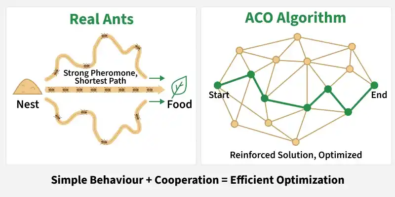
Ant Colony Optimization (ACO) is a nature-inspired algorithm that learns from how real ants collectively find the shortest path to food without any central control. Instead of fixed rules, it improves solutions over time through simple behaviour and cooperation making it effective for complex optimization problems. In nature, ants follow a simple process like:

• They move randomly and leave a pheromone trail
• Shorter paths gather pheromones faster
• More ants follow stronger trails
• Over time, the shortest path becomes dominant

Key Components

Ant Colony Optimization is built on a few core components that work together to guide the search toward optimal solutions.

1. Ants: Simple agents that explore the problem space and construct solutions step by step.
2. Pheromone trails: Numerical values that store past experience and indicate which paths are more promising.
3. Heuristic information: Problem specific knowledge such as distance, cost or time that helps ants make informed decisions.
4. Probability based movement: Ants choose paths using probabilities influenced by pheromones and heuristic values, rather than fixed rules.
5. Pheromone evaporation: Pheromone levels gradually decrease over time, preventing premature convergence and encouraging continued exploration.

How it Works

Ant Colony Optimization operates through an iterative loop that progressively refines solutions based on collective learning.

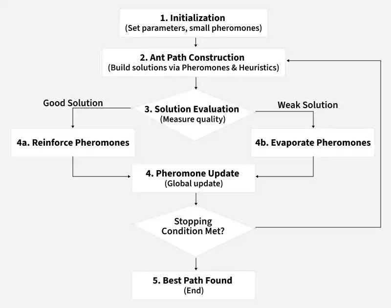
1. Initialization: Set initial parameters and assign small pheromone values to all paths.
2. Ant path construction: Each ant builds a solution by moving through the problem space based on pheromones and heuristic information.
3. Solution evaluation: The quality of each solution is measured using a fitness or cost function.
4. Pheromone update: Good solutions receive more pheromone reinforcement, while pheromones on other paths evaporate.
5. Iteration until best path is found: The process repeats until a stopping condition is met or the best path is discovered.

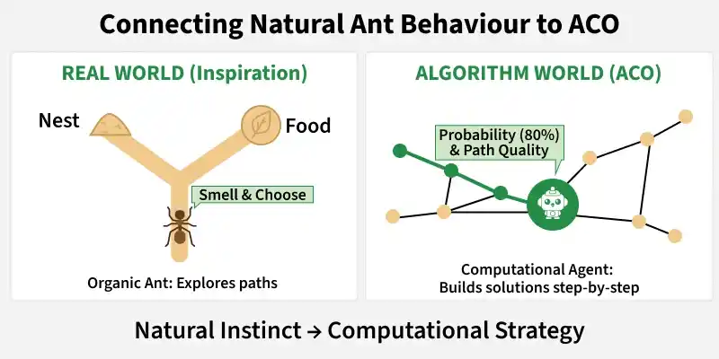
Turning Ant Behaviour into a Problem Solving Strategy

Ant Colony Optimization converts the natural behaviour of ants into a computational problem solving framework, where simple agents collectively build high quality solutions.

1. Ants as agents: In ACO, each ant is a simple computational agent that constructs a solution step by step, similar to how real ants explore routes.
2. Pheromones as memory: Pheromones are numerical values assigned to paths, representing how effective those paths were in previous solutions.
3. Nodes and paths: Nodes represent possible states or locations, while paths represent transitions between them, similar to routes between a nest and food.
4. Decision making: Ants select paths probabilistically, considering both pheromone strength and path quality instead of following fixed rules.

Parameters in Ant Colony Optimization

The performance and behaviour of Ant Colony Optimization depend on a few key parameters that balance exploration and exploitation.

1. Number of ants: Determines how many solutions are explored in each iteration. More ants improve exploration but increase computation.
2. Pheromone importance: Controls how strongly ants follow previously successful paths. Higher importance means more exploitation of known good solutions.
3. Heuristic importance: Defines how much ants rely on problem specific information such as distance or cost while choosing paths.
4. Evaporation rate: Decides how quickly pheromone values fade over time. A higher rate encourages exploration, while a lower rate favours stability.

How Ants Discover the Shortest Path

Ant Colony Optimization is inspired by how real ants search for food and collectively discover the shortest path without any central control. Their behaviour can be understood through a few simple ideas:

1. Random exploration: Ants initially move in different directions, exploring multiple possible paths.
2. Pheromone trails: When an ant finds food, it returns while leaving a chemical trail that guides other ants.
3. Shorter paths strengthen faster: Ants on shorter routes return more quickly and deposit pheromones more often, while longer paths fade due to evaporation.
4. Indirect communication: Ants coordinate through pheromone signals rather than a leader and is known as stigmergy.

Calculating the Shortest Path

1. Probability of Choosing the Next Path

An ant does not randomly choose a path. It selects the next node using probability.

P_{ij} = \frac{(\tau_{ij})^{\alpha} \cdot (\eta_{ij})^{\beta}}{\sum (\tau_{ik})^{\alpha} \cdot (\eta_{ik})^{\beta}}

• \tau_{ij}: pheromone on path i to j
• \eta_{ij}: how good the path looks (usually shorter distance)
• \alpha: importance of pheromone
• \beta: importance of distance

2. Heuristic Value (Distance Information)

Heuristic value represents how good a path looks based on distance. For shortest path problems:

\eta_{ij} = \frac{1}{d_{ij}}

• d_{ij}: distance between nodes i and j
• Smaller distance: larger heuristic value

This formula helps ants prefer shorter paths while making decisions.

3. Pheromone Update Rule

After all ants complete their paths, pheromones are updated:

\tau_{ij} = (1 - \rho)\tau_{ij} + \Delta\tau_{ij}

• Old pheromone partially evaporates
• New pheromone is added on good paths
• \rho: evaporation rate (between 0 and 1)

4. Pheromone Added by an Ant

Each ant adds pheromone based on path quality:

\Delta\tau_{ij} =\begin{cases}\frac{Q}{L} & \text{if the path is used} \\0 & \text{otherwise}\end{cases}

• Q: constant value
• L: total length of the path
• Shorter path: more pheromone added

Implementation

Here we Implement and Visualize Ant Colony Optimization for the Traveling Salesman Problem. It is a classic optimization problem where a salesman must visit each city exactly once and return to the starting city while minimizing the total travel distance. It aims to find the shortest possible route among all possible city permutations.

Step 1: Importing Required Libraries

Here we use:

• NumPy for handling matrices and performing numerical calculations like distances and pheromone values.
• Random for selecting starting cities and making random or probability based choices.
• Matplotlib for visualizing matrices and results in a clear graphical format.

import numpy as np
import random
import matplotlib.pyplot as plt

Step 2: Here we define the Distance Matrix

Here we define the distance matrix, where each value shows the cost between two cities (0 means same city) and n_cities automatically calculates how many cities are in the problem.

distances = np.array([
    [0, 2, 9, 10, 7],
    [2, 0, 6, 4, 3],
    [9, 6, 0, 8, 5],
    [10, 4, 8, 0, 6],
    [7, 3, 5, 6, 0]
])

n_cities = len(distances)

Step 3: Defining Hyperparameters

Here we set the main control values of the algorithm:

• alpha: how much importance is given to pheromone (past experience).
• beta: how much importance is given to distance (shorter paths preferred).
• evaporation: how quickly old pheromone fades (forgetting factor).
• Q: amount of pheromone deposited.
• n_ants: number of ants searching for solutions.
• n_iterations: number of learning cycles.

n_ants = 10
n_iterations = 50
alpha = 1
beta = 2
evaporation = 0.5
Q = 100

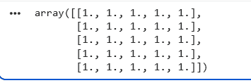
Step 4: Initialize Pheromone Matrix

Here we initialize the pheromone matrix with all values set to 1, meaning every path starts with equal importance and there is no initial bias which allows the algorithm to freely explore all possible paths in the beginning.

pheromone = np.ones((n_cities, n_cities))
pheromone

Output:

Step 5: Calculating Distance

Here we calculate the total travel distance of a given path by adding the distance between each consecutive city, and finally adding the distance from the last city back to the starting city to complete the tour (as required in TSP).

def calculate_distance(path):
    return sum(distances[path[i]][path[i+1]] 
               for i in range(len(path)-1)) \
           + distances[path[-1]][path[0]]

Step 6: Initializing Global Best Tracking parameters

We start by setting the best distance to infinity so that any valid path found will automatically be better. The global_best_path stores the best tour discovered so far.

• Ensures the algorithm keeps track of the overall best solution
• Prevents losing a better path found in earlier iterations

global_best_distance = float("inf")
global_best_path = None

Step 7: Optimization Process

• This is the main learning loop. In every iteration, each ant builds a full tour starting from a random city.
• The next city is chosen using probability based on pheromone (\tau ) and distance (\eta ), controlled by \alpha and \beta . After completing the tour, total distance is calculated.
• If a better path is found, the global best solution is updated. This is the core logic of ACO.

for iteration in range(n_iterations):

    all_paths = []
    all_distances = []

    for ant in range(n_ants):

        visited = [random.randint(0, n_cities - 1)]

        while len(visited) < n_cities:
            current = visited[-1]
            probabilities = []

            for city in range(n_cities):
                if city not in visited:
                    tau = pheromone[current][city] ** alpha
                    eta = (1 / distances[current][city]) ** beta
                    probabilities.append(tau * eta)
                else:
                    probabilities.append(0)

            probabilities = np.array(probabilities)
            probabilities /= probabilities.sum()

            next_city = np.random.choice(range(n_cities), p=probabilities)
            visited.append(next_city)

        distance = calculate_distance(visited)

        all_paths.append(visited)
        all_distances.append(distance)

        if distance < global_best_distance:
            global_best_distance = distance
            global_best_path = visited

Step 8: Evaporation of Pheromone

Here we reduce all pheromone values by multiplying them with 1 - \rho , where \rho is the evaporation rate. This prevents pheromone from increasing indefinitely and avoids over favouring one path too early. It helps maintain exploration in the system.

pheromone *= (1 - evaporation)

Step 9: Update the Pheromones

After all ants complete their tours, pheromone is added to the paths they used. The amount added depends on the tour length ,shorter paths receive more pheromone.

for path, dist in zip(all_paths, all_distances):
    for i in range(len(path) - 1):
        pheromone[path[i]][path[i+1]] += Q / dist
        pheromone[path[i+1]][path[i]] += Q / dist

    pheromone[path[-1]][path[0]] += Q / dist
    pheromone[path[0]][path[-1]] += Q / dist

Step 10: Printing Final Result

• Here we display the final best tour found by the algorithm along with its total distance.
• It shows the optimal path discovered after all iterations and confirms the best solution achieved by the colony.

print("Best Path:", global_best_path)
print("Best Distance:", global_best_distance)

Output:

Step 11: Visualizing Pheromone Matrix

plt.figure()
sns.heatmap(np.ones((n_cities, n_cities)), annot=True, cmap="viridis")
plt.title("Initial Pheromone Matrix")
plt.show()

plt.figure()
sns.heatmap(pheromone, annot=True, cmap="viridis")
plt.title("Final Pheromone Matrix")
plt.show()

Output:

In the initial matrix, every value is 1. This means:

• All paths between cities have equal importance.
• There is no preference for any route.
• The algorithm starts in pure exploration mode.

In the final matrix, values are no longer equal. Some edges now have very high values like 22, 24, 21, etc while others are much lower. This means:

• Paths with higher values were used more often.
• These paths likely belong to shorter and better tours.
• The algorithm has reinforced strong routes over time.

For example: The connection between city 1 and city 4 has a value of 24 which is highly preferred and Edges like 0–1, 0–2, 2–4 are also strongly reinforced.

You can download the code from here

Applications

Ant Colony Optimization is widely applied to real world optimization problems where discovering efficient paths or schedules is challenging.

1. Shortest path problems: Finding the most efficient route between two points.
2. Network routing: Optimizing data transmission paths in communication networks.
3. Scheduling: Allocating tasks, resources or time slots efficiently.
4. Traveling Salesman Problem (TSP): Determining the shortest possible route that visits all locations once.

Advantages

1. Works well for complex problems: It can handle large and complicated search spaces where traditional methods struggle.
2. Adaptive and flexible: The algorithm continuously learns from previous solutions and adapts over time.
3. Avoids getting stuck early: Pheromone evaporation and probabilistic choices help prevent premature convergence.
4. Suitable for dynamic environments: It can adjust when conditions change making it effective for real world problems.

Limitations

1. Can be slow for large problems: Performance may decrease as the problem size grows and more iterations are required.
2. Parameter tuning is important: Poor parameter choices can lead to slow convergence or weak solutions.
3. Not always guaranteed optimal solution: ACO aims for high quality solutions but does not always guarantee the absolute best one.