Hopfield Neural Network

A Hopfield Network is a type of recurrent neural network designed to store and recall patterns by mimicking associative memory in the human brain. It works by repeatedly updating interconnected neurons until the system settles into a stable state that represents a stored pattern. This makes it especially useful for recovering complete information from partial or noisy inputs.

• Single-layer network where each neuron is connected to every other neuron
• Input and output sizes are the same (auto-associative model)
• Uses symmetric weights with no self-connections
• Converges to a stable state through an energy minimization process

Types of Hopfield Network

Hopfield Networks are classified based on how neuron outputs are represented and how the network dynamics evolve over time.

1. Discrete Hopfield Network

A Discrete Hopfield Network is a fully interconnected recurrent neural network where each neuron is connected to every other neuron (except itself). The network updates neuron states in discrete steps and produces finite, distinct outputs.

• Functions as an auto-associative memory system that updates neurons iteratively (synchronously or asynchronously).
• Converges to a stable equilibrium state through energy minimization.
• Has limited storage capacity (0.15n patterns) and may generate spurious states when overloaded.

Discrete networks operate in two possible representations:

• Binary Representation: Output values are 0 or 1
• Bipolar Representation: Output values are -1 or +1

The weight matrix in a discrete Hopfield network follows two important rules:

w_{ij}=w_{ji} (Symmetric weights)

w_{ii}=0 (No self-connections)

These properties ensure the existence of a well-defined energy function, which guarantees convergence to a stable state.

2. Continuous Hopfield Network

A Continuous Hopfield Network differs from the discrete version in that neuron outputs are not limited to fixed values. Instead outputs vary continuously between 0 and 1.

• Operates in continuous time and is governed by differential equations.
• Energy function decreases smoothly over time, ensuring stable convergence.
• Well suited for constrained optimization problems with smoother dynamics than discrete networks.

Architecture of Hopfield Network

The Hopfield Network is a single-layer fully connected recurrent network where neurons update through feedback until a stable state is reached. Its symmetric structure enables associative memory and energy-based convergence. The core structural features of a Hopfield Network are:

• Fully Connected Network: Every neuron is connected to all other neurons in the network.
• No Self-Connections: A neuron does not connect to itself.
• Symmetric Weights: The weight matrix is symmetric.
• State Preservation: Each neuron maintains its current state until it is selected for updating.
• Asynchronous Updating: One neuron is selected and updated at a time, improving stability and ensuring convergence.

For a network with n neurons:

• X = [x_1, x_2, \ldots, x_n]: Input to the n given neurons
• Y = [y_1, y_2, \ldots, y_n]: Output obtained from the n given neurons
• W_{ij}: denotes the connection strength between neuron i and neuron j

How Hopfield Networks Learn and Recall Patterns

Training a Hopfield Network means storing patterns in the weight matrix using the Hebbian learning rule. After training, the network can recall stored patterns from partial or noisy inputs through an iterative testing process.

Training Algorithm

The Hopfield Network stores patterns using the Hebbian learning rule, which strengthens connections between neurons that activate together.

For storing a set of P input patterns the weight matrix is computed using the Hebbian outer-product rule.

S^{(p)} = \left[ s_1^{(p)},\, s_2^{(p)},\, \ldots,\, s_n^{(p)} \right], \quad p = 1, 2, \ldots, P

Here s_{i}^{(p)} is the state of the i-th neuron in that p-th pattern

Case 1: Binary Patterns (0/1)

For binary patterns, values are first converted into bipolar form before applying the Hebbian rule.

w_{ij} = \sum_{p=1}^{P} \left( 2s_i^{(p)} - 1 \right)\left( 2s_j^{(p)} - 1 \right), \quad i \ne j

Here

• (2s_i^{(p)} - 1) converts binary values (0,1) into bipolar values (-1,+1).
• Self-connections are removed by setting w_{ii}

Case 2: Bipolar Patterns (-1/+1)

For bipolar patterns, weights are directly computed using the outer-product learning rule.

w_{ij} = \sum_{p=1}^{P} s_i^{(p)} \, s_j^{(p)}, \quad i \ne j

Here s_i^{(p)} \in \{-1, +1\}and the weights are symmetric(w_{ij}=w_{ji})

Testing (Recall) Algorithm

After training, the Hopfield Network recalls stored patterns by iteratively updating neuron states until convergence to a stable state (energy minimum). Asynchronous updating is typically used to guarantee convergence.

Step 1: Initialize the Network

Set the initial state equal to the input vector

Step 2: Compute Net Input

For the selected neuron i, compute the net input:

y_{in_i} = \sum_{j=1}^{n} w_{ij} y_j

Step 3: Apply Activation Function

For binary representation (0/1):

y_i =\begin{cases}1 & \text{if } y_{in_i} > \theta_i \\y_i & \text{if } y_{in_i} = \theta_i \\0 & \text{if } y_{in_i} < \theta_i\end{cases}

For bipolar representation (-1/+1):

y_i =\begin{cases}+1 & \text{if } y_{in_i} \ge 0 \\-1 & \text{if } y_{in_i} < 0\end{cases}

Step 4: Update and Feedback

In asynchronous updating, one neuron is updated at a time by replacing its old state with the new value and the updated output is then fed back to all other neurons in the network.

Step 5: Check for Convergence

The network is said to have converged when no neuron changes its state during a complete update cycle, indicating that a stable state (local energy minimum) has been reached.

Energy Function in Hopfield Network

Energy function (Lyapunov function) assigns an energy value to every possible state of the network. During the updating process, the energy either decreases or remains constant, ensuring that the network eventually converges to a stable state (local minimum).

1. Energy Function in Discrete Hopfield Network

For a network with symmetric weights and no self-connections, the energy function is defined as:

E = -\frac{1}{2} \sum_{i=1}^{n} \sum_{j=1}^{n} w_{ij} x_i x_j + \sum_{i=1}^{n} \theta_i x_i

where

• w_{ij}: weight between neuron i and neuron j
• x_{i},x_{j}: states of neurons
• \theta_{i}: threshold of neuron i

In asynchronous updating, the energy never increases and the network converges to a stable memory state at a local minimum.

2. Energy Function in Continuous Hopfield Network

In the continuous network neuron outputs vary smoothly and the energy function is defined as:

E = -\frac{1}{2} \sum_{i=1}^{n} \sum_{j=1}^{n} w_{ij} v_i v_j + \sum_{i=1}^{n} \theta_i v_i

where v_{i} represent continuous output of neuron i.

Convergence Condition

For continuous dynamics, convergence is guaranteed if:

\frac{dE}{dt} \leq 0

This means the energy decreases over time. The neuron dynamics are governed by:

\frac{du_i}{dt} = -\frac{u_i}{\tau} + \sum_{j=1}^{n} w_{ij}v_j + \theta_i

where

• u_{i}: internal state
• \tau: time constant
• v_{i}=g(u_{i}): activation function

Step By Step Implementation

Here we implement Hopfield Neural Network

Step 1: Import Required Libraries

Here we import all the necessary libraries for building and running the Hopfield Network

!pip install scikit-image tqdm

import numpy as np
from matplotlib import pyplot as plt
from skimage.filters import threshold_mean
from tqdm import tqdm
from tensorflow.keras.datasets import mnist

Step 2: Define Hopfield Network and Train Weights

Here we define the Hopfield Network class and implement the weight training method.

• We calculate the weight matrix using Hebbian learning with mean-centering.
• The diagonal is set to 0 to avoid self-connections.

class HopfieldNetwork:
    def train_weights(self, train_data):
        self.num_neuron = train_data[0].size  # number of neurons
        rho = np.mean([np.sum(d) for d in train_data])  # mean activity
        W = sum(np.outer(d - rho, d - rho) for d in train_data)  # Hebbian sum
        np.fill_diagonal(W, 0)  # no self-connection
        self.W = W / len(train_data)  # normalize by number of patterns

Step 3: Predict Patterns and Compute Energy

Here we implements pattern recall:

• The network updates neurons asynchronously or synchronously.
• Updates stop when the energy converges or max iterations are reached.
• Energy of the state is calculated to track convergence.

    def predict(self, data, num_iter=20, threshold=0, asyn=True):
        pred = []
        energies = []
        for s in tqdm(data):
            s = s.copy()
            e_list = [self.energy(s)]
            for _ in range(num_iter):
                if asyn:  # asynchronous update
                    for _ in range(self.num_neuron):
                        i = np.random.randint(self.num_neuron)
                        s[i] = np.sign(self.W[i] @ s - threshold)
                        if s[i] == 0: s[i] = 1
                else:  # synchronous update
                    s = np.sign(self.W @ s - threshold)
                    s[s == 0] = 1
                e_new = self.energy(s)
                e_list.append(e_new)
                if e_new == e_list[-2]:  # stop if energy converged
                    break
            pred.append(s)
            energies.append(e_list)
        return pred, energies
    
    def energy(self, s):
        return -0.5 * s @ self.W @ s

Step 4: Preprocess Images

Convert grayscale images into bipolar format −1,+1 using a threshold.

def preprocess(img):
    return 2*(img > threshold_mean(img)).astype(int)-1

def reshape_img(v): 
    dim = int(np.sqrt(v.size))
    return v.reshape((dim, dim))

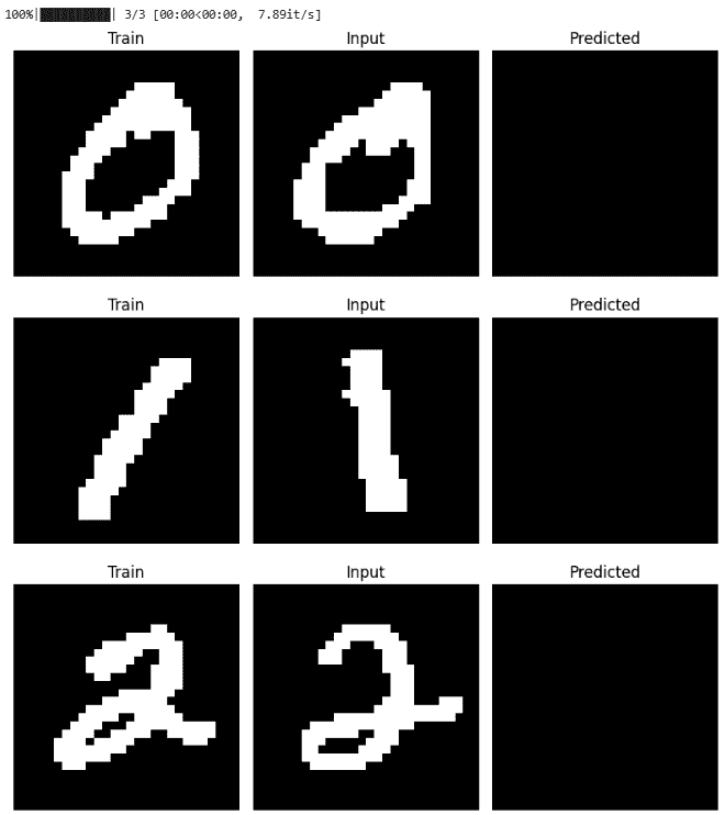
Step 5: Plot Training, Input and Predicted Images

Visual comparison between stored memory, input and network output.

def plot_results(train, test, predicted):
    train = [reshape_img(d) for d in train]
    test = [reshape_img(d) for d in test]
    predicted = [reshape_img(d) for d in predicted]
    
    fig, axes = plt.subplots(len(train), 3, figsize=(8, 3*len(train)))
    if len(train) == 1: axes = [axes]
    for i in range(len(train)):
        for j, data in enumerate([train[i], test[i], predicted[i]]):
            axes[i][j].imshow(data, cmap='gray')
            axes[i][j].axis('off')
            axes[i][j].set_title(["Train","Input","Predicted"][j])
    plt.tight_layout()
    plt.show()

Step 6: Hamming Distance

Calculate the number of differing bits between predicted patterns and stored memories.

def hamming_distance(a, b):
    return np.sum(a != b)

Step 7: Load MNIST Data and Select Training/Testing Images

Pick one image per class for training and one for testing. Preprocess them.

(x_train, y_train), _ = mnist.load_data()

train_imgs = [preprocess(x_train[y_train==i][0]) for i in range(3)]
test_imgs  = [preprocess(x_train[y_train==i][1]) for i in range(3)]

flattened_train_imgs = [img.flatten() for img in train_imgs]
flattened_test_imgs = [img.flatten() for img in test_imgs]

Step 8: Train the Hopfield Network

Train the weight matrix using the flattened training images.

model = HopfieldNetwork()
model.train_weights(flattened_train_imgs)

Step 9: Predict and Track Energy

Run the network on test images with asynchronous updates and record energy convergence.

predicted, energies = model.predict(flattened_test_imgs, num_iter=20, asyn=True)

Step 10: Visualize Results

Compare training images, inputs and outputs.

plot_results(train_imgs, test_imgs, predicted)

Output:

Step 11: Plot Energy Convergence

Show how energy decreases during iterative updates.

for i, e_list in enumerate(energies):
    plt.plot(e_list, marker='o')
    plt.title(f'Energy Convergence for Test Image {i}')
    plt.xlabel('Iteration')
    plt.ylabel('Energy')
    plt.grid(True)
    plt.show()

Output:

These plots how the energy of each test image changes over iterations in the Hopfield Network.

• The y-axis shows the energy value and the x-axis shows the iteration number.
• A decreasing or stable energy curve indicates the network is converging to a stable memory state

You can download full code from here