Decision Tree Algorithms are widely used supervised machine learning methods for both classification and regression tasks. They split data based on feature values to create a tree-like structure of decisions, starting from a root node and ending at leaf nodes that provide predictions.
- Decision trees are non-parametric models that can handle both numerical and categorical features without assuming any specific data distribution.
- They use splitting measures such as Information Gain, Gini Index or Variance Reduction to determine the best feature for dividing the data.
- Decision trees also act as building blocks for powerful ensemble models like Random Forest and Gradient Boosting.
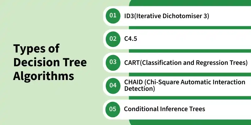
1. ID3 (Iterative Dichotomiser 3)
ID3 (Iterative Dichotomiser 3) is a decision tree learning algorithm used for solving classification problems. It builds the tree using a top-down, greedy approach by selecting the attribute that provides the highest Information Gain which is calculated using entropy.
- ID3 mainly works with categorical attributes and recursively splits the data until the nodes become pure or no attributes remain.
- It is simple and easy to interpret but can overfit the training data and does not handle continuous features directly.
How ID3 Builds the Decision Tree
The ID3 algorithm constructs a decision tree by selecting the attribute that best splits the dataset at each step. It uses Entropy and Information Gain to measure impurity and determine the most informative feature for splitting the data.
Step 1: Initialize Root Node
The entire dataset is placed at the root node containing all training samples.
Step 2: Calculate Entropy
Entropy measures the amount of randomness or impurity in a dataset. If all data points belong to the same class, entropy is 0 (pure node). If the data is evenly distributed among classes, entropy is higher, indicating more disorder.
H(D) = -\sum_{i=1}^{n} p_i \log_2(p_i)
where
H(D) : entropy of dataset Dp_{i} : probability of class i in the dataseti : number of classes
Step 3: Compute Information Gain
Information Gain measures how much entropy decreases after splitting the dataset based on a particular feature. The feature with the highest Information Gain is selected for the split because it provides the most useful information for classification.
Information Gain = H(D) - \sum_{v=1}^{V} \frac{|D_v|}{|D|} H(D_v)
where
D : original datasetD_v : subset of the dataset after splitting on a feature value v|D_v| : number of samples in subset v|D| : total number of samples in the datasetV : number of possible values of the feature
Step 4: Select Best Attribute and Split
The attribute with the highest Information Gain is selected, and the dataset is divided into subsets based on its values.
Step 5: Repeat Recursively
The same process continues for each subset until the node becomes pure or no attributes remain for further splitting, forming the final leaf nodes of the tree.
Limitations
- ID3 tends to overfit the training data, especially when the tree becomes very deep.
- It cannot directly handle continuous attributes without preprocessing.
- The algorithm may be biased toward features with many unique values.
Refer: Iterative Dichotomiser 3 (ID3) Algorithm From Scratch
2. C4.5
C4.5 is an improved extension of the ID3 algorithm. It is designed to overcome several limitations of ID3, such as handling continuous attributes, managing missing values and reducing bias toward attributes with many values by using Gain Ratio instead of Information Gain.
- Uses Gain Ratio as the splitting criterion to reduce bias toward attributes with many distinct values.
- Can handle both categorical and continuous attributes, making it more flexible than ID3.
- Applies post-pruning techniques to simplify the tree and reduce overfitting.
How C4.5 Builds the Decision Tree
C4.5 builds the decision tree by selecting the best attribute for splitting using Gain Ratio, which helps produce balanced splits and reduce bias toward attributes with many values.
Step1: Initialize Root Node
The entire dataset is placed at the root node containing all training samples.
Step 2: Compute Information Gain
Information Gain is calculated for each attribute to measure how much entropy decreases after a split.
Step 3: Compute Split Information
Split Information measures how the dataset is distributed across different branches after splitting.
\text{Split Information} = -\sum_{i=1}^{n} \frac{|D_i|}{|D|} \log_2 \left( \frac{|D_i|}{|D|} \right)
Step 4: Calculate Gain Ratio
Gain Ratio normalizes Information Gain to avoid bias toward attributes with many distinct values.
\text{Gain Ratio} = \frac{\text{Information Gain}}{\text{Split Information}}
Step 5: Select Best Attribute and Split
The attribute with the highest Gain Ratio is selected and the dataset is divided into subsets based on its values.
Step 6: Repeat Recursively
The same process continues for each subset until nodes become pure or no attributes remain, followed by post-pruning to simplify the tree.
Limitations
- C4.5 can still overfit noisy datasets, even though pruning reduces this issue.
- The algorithm may become computationally expensive when dealing with very large datasets or many features.
- Decision trees generated by C4.5 can become complex and difficult to interpret when the tree grows too deep.
3. CART (Classification and Regression Trees)
CART is a widely used decision tree algorithm that can handle both classification and regression problems. CART builds binary decision trees by repeatedly splitting the dataset into two subsets based on the most informative feature.
- Works for both classification and regression tasks.
- Uses Gini Impurity for classification and variance reduction for regression.
- Always produces binary trees, meaning each internal node splits into exactly two child nodes.
How CART Builds the Decision Tree
CART constructs the decision tree by repeatedly selecting the best feature and split point that reduces impurity in the dataset. The algorithm evaluates different splits and chooses the one that creates the most homogeneous subsets.
Step 1: Initialize Root Node
The process begins with the entire dataset placed at the root node. This node contains all training samples before any splitting occurs.
Step 2: Calculate Gini Impurity (for Classification)
CART measures how impure the dataset is using Gini Impurity, which estimates the probability of incorrectly classifying a randomly chosen sample.
Gini(D) = 1 - \Sigma^n _{i=1}\; p^2_{i}
where
Step 3: Evaluate Possible Splits
The algorithm examines different features and possible split points to determine how well they divide the data into more homogeneous groups.
Step 4: Select the Best Split
The feature and split point that produce the lowest Gini impurity (for classification) or maximum variance reduction (for regression) are selected to divide the dataset.
Step 5: Create Binary Branches
CART always creates binary splits, meaning each node is divided into exactly two child nodes (left and right), which simplifies the tree structure.
Step 6: Repeat Recursively
The same process continues for each subset, splitting the data until stopping criteria are met such as reaching pure nodes or a minimum number of samples.
Limitations
- CART can overfit training data if the tree grows too deep.
- The algorithm can be sensitive to small changes in the dataset, leading to different tree structures.
- Large trees may become computationally expensive and harder to interpret.
Refer: Implementing CART (Classification And Regression Tree) in Python
4. CHAID (Chi-Square Automatic Interaction Detection)
CHAID is a decision tree algorithm mainly used for classification and regression analysis, especially when dealing with categorical variables. It builds trees by using statistical chi-square tests to identify the feature that has the strongest relationship with the target variable.
- Uses Chi-Square statistical tests to determine the best feature for splitting the dataset.
- Works well with categorical variables and can handle datasets with many categories.
- Unlike CART, CHAID can create multi-way splits, meaning a node can have more than two branches.
- This approach makes CHAID particularly useful for exploratory data analysis and large datasets with many categorical features.
How CHAID Builds the Decision Tree
CHAID constructs the decision tree by analyzing the statistical relationship between each feature and the target variable using the chi-square test.
Step 1: Initialize Root Node
The entire dataset is placed at the root node, which contains all training samples before any splitting occurs.
Step 2: Perform Chi-Square Test
For each categorical feature, CHAID calculates the Chi-Square statistic to measure the strength of association between the feature and the target variable.
X^2 = \Sigma \frac{(O_{i} - E_{i})^2}{E_{i}}
where:
O_i represents the observed frequencyE_i represents the expected frequency in each category.
Step 3: Select the Best Feature
The feature with the highest chi-square value (indicating the strongest relationship with the target variable) is selected for splitting the dataset.
Step 4: Create Multi-Way Branches
CHAID divides the dataset into multiple subsets based on the categories of the selected feature, creating several branches from a single node.
Step 5: Repeat Recursively
The algorithm continues the same process for each subset until stopping criteria are met, such as reaching statistically insignificant splits or minimum node size.
Prediction Using CHAID
- For Classification: The algorithm assigns a class label to a new data point by following the path from the root node to a leaf node and the class of that leaf node becomes the prediction.
- For Regression: The predicted value is typically the average of the target variable values within the leaf node.
Limitations
- CHAID can require large sample sizes to produce reliable statistical results.
- It may struggle with continuous variables, which often need to be converted into categories.
- The tree can become large and complex when the dataset contains many categorical values.
5. Conditional Inference Trees
Conditional Inference Trees are decision tree models that use statistical hypothesis tests to select the best feature for splitting the dataset. Unlike algorithms such as CART, they use permutation-based tests to reduce bias toward variables with many categories. This makes them useful when working with datasets containing a mix of categorical and continuous variables.
- Uses statistical hypothesis tests to select splitting features instead of impurity measures like Gini or Information Gain.
- Reduces selection bias toward variables with many categories or unique values.
How Conditional Inference Trees Build the Decision Tree
Conditional Inference Trees construct the tree using a recursive partitioning process based on statistical significance tests.
Step 1: Initialize Root Node
The entire dataset is placed at the root node, containing all training samples before any splitting occurs.
Step 2: Test Association Between Features and Target
At each node, the algorithm performs statistical tests to evaluate the relationship between each predictor variable and the target variable. For example, it may use Chi-square tests for categorical variables or F-tests for continuous variables.
Step 3: Select the Most Significant Feature
The feature with the strongest statistically significant association with the target variable (lowest p-value) is selected as the splitting variable.
Step 4: Determine the Best Split Point
The algorithm determines the optimal way to divide the data based on the selected feature, creating new subsets that maximize the statistical difference between groups.
Step 5: Repeat Recursively
The process is repeated for each subset until no statistically significant relationship remains or predefined stopping criteria are met.
Advantages
- Reduces variable selection bias, which is common in traditional decision tree algorithms.
- Provides statistically reliable splits based on hypothesis testing.
- Works well with mixed data types and complex datasets.
Limitations
- The statistical testing process can make the algorithm computationally slower than traditional decision trees.
- Trees may become complex when dealing with large datasets.
- Interpretation can sometimes be less intuitive compared to simpler decision tree methods
ID3 vs C4.5 vs CART vs CHAID vs Conditional Inference Trees
Algorithm | Splitting Method | When to Use |
|---|---|---|
ID3 | Entropy and Information Gain on categorical features only | Simple classification with categorical data |
C4.5 | Gain Ratio handles continuous and categorical features applies pruning | Mixed data types with better generalization than ID3 |
CART | Gini Impurity for classification variance reduction for regression binary splits | Classification and regression tasks on tabular data |
CHAID | Chi-Square test multi-way splits for categorical features | Large datasets with many categorical variables |
Conditional Inference Trees | Statistical hypothesis and permutation tests unbiased splits | Mixed data types and unbiased feature selection |