System of Linear Equations

A system of linear equations is a set of two or more linear equations involving the same set of variables. Each equation represents a straight line or a plane, and the solution to the system is the set of values for the variables that satisfy all equations simultaneously. This system can have one solution (consistent and independent), no solution (inconsistent), or infinitely many solutions (dependent).

Here is a simple example of a system of linear equations:

General Form

A system of linear equations consists of multiple linear equations involving the same set of variables. It can be represented as follows:

\begin{aligned}a_{11}x_1 + a_{12}x_2 + a_{13}x_3 + \dots + a_{1n}x_n &= b_1 \\a_{21}x_1 + a_{22}x_2 + a_{23}x_3 + \dots + a_{2n}x_n &= b_2 \\&\vdots \\a_{n1}x_1 + a_{n2}x_2 + a_{n3}x_3 + \dots + a_{nn}x_n &= b_n\end{aligned}

This represents a system of n linear equations in n variables x₁, x₂, x₃,…., x_n.

Where,

• a₁₁, a₁₂, …, a₂₁, a₂₂,…, a_n1, a_n2,…, a_nn are the coefficients of variables, x₁, x₂,…., x_n.
• b₁ + b₂ + b₃ + …. + b_n are the constants on the right-hand side of each equation.

Matrix Equation

These equations can be written in matrix form as AX = B, where:

• A is the coefficient matrix,
• X is the column vector of variables \left[ x_1, x_2, x_3, \dots, x_n \right]^T ,
• B is the column vector of constants \left[ b_1 + b_2 + b_3 + \dots + b_n \right]^T .

A =\begin{bmatrix} a_{11} & a_{12} & a_{13}& \cdots & a_{1n} \\ a_{21} & a_{22} & a_{23}& \cdots & a_{2n} \\ a_{31} & a_{32} & a_{33}&\cdots & a_{3n}\\\vdots & \vdots & \vdots & \vdots & \vdots \\ a_{m1} & a_{m2} & a_{m3} &\cdots & a_{mn} \end{bmatrix} , X = \begin{bmatrix} x_1 \\ x_2 \\ x_3 \\\vdots \\x_{n}\end{bmatrix} and\ B = \begin{bmatrix} b_1 \\ b_2 \\ b_3 \\\vdots \\b_{m}\end{bmatrix}

Solving the system involves finding the values of x₁, x₂, x₃,…., x_n that satisfy all equations simultaneously.

Types of system of linear equations

1. Homogeneous System (AX = 0)
2. Non-Homogeneous System (AX = B)

The solution of these systems depends on the rank of the coefficient matrix A and the rank of the augmented matrix [A :B].

1) System of Homogeneous linear equations AX = 0

1. X = 0 is always a solution: means all the unknowns have same value as zero. (This is also called trivial solution)
2. If P(A) = number of unknowns : Unique solution (P(A) = Rank of matrix A).
3. If P(A) < number of unknowns : Infinite number of solutions.

Since a homogeneous system always has at least one solution (X = 0), it is always consistent.

Example of Homogeneous System in three variable:

x + y - z = 0
x + y + z = 0
x - y + 2z = 0

2) System of Non-Homogeneous linear equations AX = B

1. If P[A:B] ≠ P(A), No solution.
2. If P[A:B] = P(A) = Number of unknown variables, unique solution.
3. If P[A:B] = P(A) ≠ Number of unknown, infinite number of solutions.

Example of Non - Homogeneous System in three variable

x + y - 2z = 6
x - 6y + z = 9
2x - y + 2z = 2

Geometric interpretation

For a system of two linear equations with two variables (x and y), solving the system involves finding the point of intersection of the two lines represented by the equations on the xy-plane. There are three possibilities:

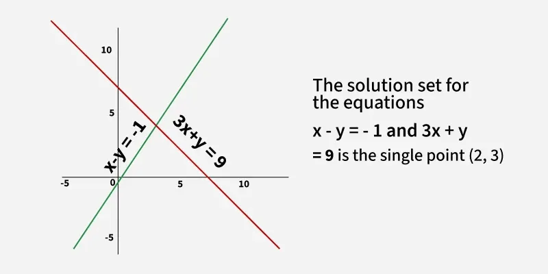
1) The lines intersect at one point: This point is the unique solution to the system.

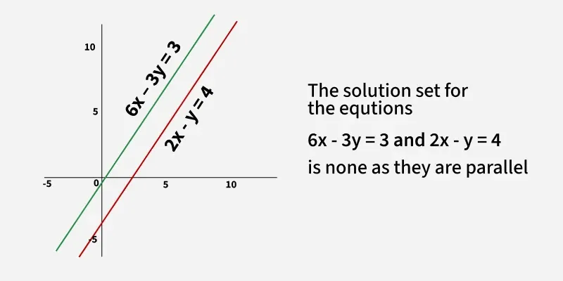
2) The lines are parallel: They never intersect, so there is no solution. The system is called inconsistent.

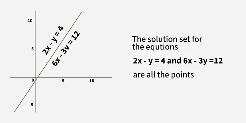
3) The lines are coincident: They are the same line, so every point on the line is a solution. There are infinitely many solutions.

The solution set to a system of two linear equations in two variables can be a single point, the empty set (no solution) or an infinite set of points (a line).

Method for Solving System of Linear Equations

The method of solving a system of linear equation are broadly classified into direct methods, which give the exact solution in a finite number of steps(like Gaussian elimination) and indirect(iterative) method that are as follow:

Direct Methods:

Direct methods provide an exact solution to the system of linear equations in a finite number of steps. They are typically preferred for smaller systems or when an exact solution is needed.

1. Cramer's Rule: This is a mathematical theorem used to solve systems of linear equations using determinants, providing a straightforward formula for each variable in the system.
2. Inverse Method: This involves finding the inverse of the coefficient matrix in a system of linear equations and multiplying it by the constant vector to solve for the variables.
3. Gauss Elimination Method: This systematically eliminates variables from a system of linear equations using row operations to transform the system into an upper triangular matrix for easier back substitution.
4. LU Decomposition Method of Factorization: This a matrix into the product of a lower triangular matrix (L) and an upper triangular matrix (U), simplifying the solution of linear systems by solving two simpler triangular systems.

Indirect Methods:

Indirect methods (also called iterative methods) are generally used for solving larger systems where direct methods may be computationally expensive or inefficient. These methods generate approximations to the solution, and the accuracy improves as the iterations progress.

1. Jacobi Method: Each equation is solved for one variable, using the values of the other variables from the previous iteration. The iteration is continued until the solution converges to a certain tolerance.
2. Gauss-Seidel Method: This is analogous to the Jacobi method, but in the Gauss-Seidel method, the new calculated values of the variables are used directly in the following iteration. This generally results in quicker convergence than the Jacobi method.
3. Successive Over-Relaxation (SOR): It is a development of the Gauss-Seidel method. It adds a relaxation factor for accelerating the convergence process. The new variable values are updated with a weighted average of the new value and the value from the previous iteration.

Applications of System of Linear Equations

Systems of linear equations are widely used in various engineering disciplines:

• Structural Analysis: In civil and mechanical engineering, they are used to analyze forces in structures, determine displacements and design stable frameworks.
• Electrical Circuit Analysis: In electrical engineering, Kirchhoff's laws lead to systems of linear equations that are used to analyze currents and voltages in electrical circuits.
• Control Systems: In control engineering, linear equations model dynamic systems and are used to design controllers that ensure desired system behavior.
• Optimization Problems: In industrial engineering and operations research, systems of linear equations arise in linear programming problems used to optimize production, transportation and resource allocation.

Practice Problem

Question 1: What is the type of system for the equation AX = 0?

Question 2: Which method involves using determinants to solve a system of linear equations?

Question 3: What is the geometric interpretation when two lines are coincident?

Question 4: What type of methods are used for larger systems of equations where direct methods may be inefficient?

Answer :

1. Homogeneous
2. Cramer's Rule
3. Infinite solutions
4. Indirect methods