In fields like computational biology, we often deal with wide numeric data. For example, we may have ~100 samples of hundreds of thousands or millions of features, say a 100 x 1e6 matrix.
Unfortunately, recipes, while very intuitive and clear, exhibits catastrophic speed issues, which precludes its use with such data. What's worse, there seems be super-linear scaling with increasing numbers of features (columns), which is clearly pathological.
The attached reprex demonstrates this and was adapted from a real-world task, where we wanted to pre-process a 48 x 500,000 matrix of features by mean centering and eliminating features with zero variance. Already at 50,000 features, the prep() + bake() workflow takes > 150 seconds. Add to this the problem of super-linear behavior, and we have a dealbreaker. This should be compared to ~0.3 seconds for the equivalent workflow at 50,000 features in Python using sklearn.Pipeline() with equivalent steps.
Profiling revealed that step_center() appears to assign centered columns back into a tibble one column at a time, causing repeated tibble/vctrs restoration overhead. Lion's share of the time is spent in:
[[<-.tbl_df
tbl_subassign_col
vectbl_restore
.Call(tibble_restore_impl, ...)
Reprex:
rm(list = ls())
# Reprex for slow recipes preprocessing with many numeric predictors.

library(tidyverse)
library(recipes)
#>
#> Attaching package: 'recipes'
#> The following object is masked from 'package:stringr':
#>
#>     fixed
#> The following object is masked from 'package:stats':
#>
#>     step


# Parameters --------------------------------------------------------------

set.seed(123)

sample_n <- 48L
predictor_counts <- seq(10000L, 60000L, by = 10000L)
trial_n <- 10L
zero_variance_prop <- 0.20
train_n <- 36L


# Data simulation ---------------------------------------------------------

simulate_predictor_matrix <- function(predictor_n) {
  zero_variance_n <- as.integer(round(predictor_n * zero_variance_prop))
  variable_n <- predictor_n - zero_variance_n

  zero_variance_matrix <- sample(
    c(0, 0.5, 1),
    size = zero_variance_n,
    replace = TRUE
  ) |>
    rep(each = sample_n) |>
    matrix(nrow = sample_n, ncol = zero_variance_n)

  variable_matrix <- matrix(
    stats::rbinom(
      n = sample_n * variable_n,
      size = trial_n,
      prob = rep(
        0.5 - 0.5 * cos(pi * stats::runif(variable_n)),
        each = sample_n
      )
    ),
    nrow = sample_n,
    ncol = variable_n
  ) / trial_n

  cbind(zero_variance_matrix, variable_matrix)
}


# Timing ------------------------------------------------------------------

time_recipe_preprocessing <- function(predictor_n) {
  recipe_data <- simulate_predictor_matrix(predictor_n) |>
    as.data.frame(check.names = FALSE) |>
    dplyr::mutate(outcome = seq_len(sample_n), .before = 1L)

  names(recipe_data) <- c("outcome", paste0("x_", seq_len(predictor_n)))

  train_data <- recipe_data[seq_len(train_n), ]
  assessment_data <- recipe_data[seq(from = train_n + 1L, to = sample_n), ]

  gc()

  elapsed_seconds <- system.time(
    {
      prepped_recipe <- recipes::recipe(
        x = train_data
      ) |>
        recipes::update_role(outcome, new_role = "outcome") |>
        recipes::update_role(
          tidyselect::starts_with("x_"),
          new_role = "predictor"
        ) |>
        recipes::step_zv(recipes::all_predictors()) |>
        recipes::step_center(recipes::all_predictors(), na_rm = FALSE) |>
        recipes::prep(retain = FALSE)

      recipes::bake(prepped_recipe, new_data = train_data)
      recipes::bake(prepped_recipe, new_data = assessment_data)
    }
  )[["elapsed"]]

  tibble::tibble(
    predictor_n = predictor_n,
    zero_variance_n = as.integer(round(predictor_n * zero_variance_prop)),
    elapsed_seconds = elapsed_seconds
  )
}

recipe_timing_tbl <- purrr::map_dfr(
  predictor_counts,
  time_recipe_preprocessing
)

print(recipe_timing_tbl)
#> # A tibble: 6 × 3
#>   predictor_n zero_variance_n elapsed_seconds
#>         <int>           <int>           <dbl>
#> 1       10000            2000            7.87
#> 2       20000            4000           65.4
#> 3       30000            6000          161.
#> 4       40000            8000          242.
#> 5       50000           10000          204.
#> 6       60000           12000          282.


# profvis::profvis({time_recipe_preprocessing(60000L)})


# Plot --------------------------------------------------------------------

recipe_timing_plot <- recipe_timing_tbl |>
  ggplot2::ggplot(
    ggplot2::aes(x = predictor_n, y = elapsed_seconds)
  ) +
  ggplot2::geom_point() +
  ggplot2::geom_line() +
  ggplot2::scale_x_continuous(
    labels = scales::label_number(big.mark = ",")
  ) +
  ggplot2::labs(
    x = "Number of predictor columns",
    y = "recipes::prep() + 2 x bake() elapsed time (s)"
  ) +
  ggplot2::theme_minimal()

print(recipe_timing_plot)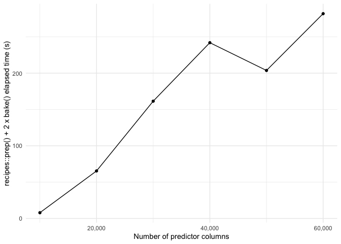
Created on 2026-05-04 with reprex v2.1.1
In fields like computational biology, we often deal with wide numeric data. For example, we may have ~100 samples of hundreds of thousands or millions of features, say a 100 x 1e6 matrix.
Unfortunately, recipes, while very intuitive and clear, exhibits catastrophic speed issues, which precludes its use with such data. What's worse, there seems be super-linear scaling with increasing numbers of features (columns), which is clearly pathological.
The attached reprex demonstrates this and was adapted from a real-world task, where we wanted to pre-process a 48 x 500,000 matrix of features by mean centering and eliminating features with zero variance. Already at 50,000 features, the
prep()+bake()workflow takes > 150 seconds. Add to this the problem of super-linear behavior, and we have a dealbreaker. This should be compared to ~0.3 seconds for the equivalent workflow at 50,000 features in Python usingsklearn.Pipeline()with equivalent steps.Profiling revealed that
step_center()appears to assign centered columns back into a tibble one column at a time, causing repeated tibble/vctrs restoration overhead. Lion's share of the time is spent in:Reprex:
Created on 2026-05-04 with reprex v2.1.1