Spearman’s Rank Correlation is a statistical measure used to find the strength and direction of association between two ranked variables. It checks how well the relationship between two variables can be described using a monotonic function.
- Works on ranks instead of actual values
- Used when data is not normally distributed
- Suitable for ordinal data
- Measures monotonic relationships, not just linear ones
Mathematical Intuition
Spearman’s Rank Correlation, denoted by ρ (rho), measures the strength and direction of association between two variables based on their ranks instead of actual values. Values range from -1 to +1
- +1: perfect positive monotonic relationship i.e if one variable increases as the other increases
- -1: perfect negative monotonic relationship i.e if one increases while the other decreases
- 0: no monotonic relationship
Monotonic Relationship means a relationship where variables move in one direction only.
Spearman's Correlation formula
\rho = 1 - \frac{6\sum d ^{2}}{n(n^2-1)}
where:
- d: difference between ranks of corresponding values
- n: total number of observation
When to Use Spearman’s Rank Correlation
- Works with non-linear data
- Data follows a monotonic trend
- Variables contain ranks or scores
- Does not assume normal distribution
- Handles ordinal data
- Dataset contains outliers
Calculating Spearman’s Rank Correlation
Step 1: Original Data
| Number | X1 | Y1 |
|---|---|---|
| 1 | 7 | 5 |
| 2 | 6 | 4 |
| 3 | 4 | 5 |
| 4 | 5 | 6 |
| 5 | 8 | 10 |
| 6 | 7 | 7 |
| 7 | 10 | 9 |
| 8 | 3 | 2 |
| 9 | 9 | 8 |
| 10 | 2 | 1 |
Step 2: Convert Data into Ranks
Ranks are assigned by sorting values in ascending order. If values are tied, the average rank is assigned.
Ranking X1:
- Sorted X1 values:
2, 3, 4, 5, 6, 7, 7, 8, 9, 10 - The two values 7 and 7 are tied → both get rank 6.5
Ranking Y1:
- Ranks are assigned using the same method.
- Sorted Y1 values:
1, 2, 4, 5, 5, 6, 7, 8, 9, 10 - The two values 5 and 5 are tied i.e both receive the average rank 4.5
Step 3: Rank Table with Differences
| No. | Rank X1 | Rank Y1 | d | d² |
|---|---|---|---|---|
| 1 | 6.5 | 4.5 | 2 | 4 |
| 2 | 5 | 3 | 2 | 4 |
| 3 | 3 | 4.5 | -1.5 | 2.25 |
| 4 | 4 | 6 | -2 | 4 |
| 5 | 8 | 10 | -2 | 4 |
| 6 | 6.5 | 7 | -0.5 | 0.25 |
| 7 | 10 | 9 | 1 | 1 |
| 8 | 2 | 2 | 0 | 0 |
| 9 | 9 | 8 | 1 | 1 |
| 10 | 1 | 1 | 0 | 0 |
\sum d^2 = 20.5
Step 4: Apply the Formula
This indicates a strong positive monotonic relationship
Calculating Spearman’s Rank Correlation in Python
Step 1: Sample Data
import pandas as pd
import seaborn as sns
import matplotlib.pyplot as plt
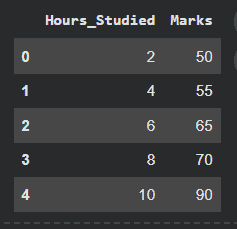
data = {
'Hours_Studied': [2, 4, 6, 8, 10],
'Marks': [50, 55, 65, 70, 90]
}
df = pd.DataFrame(data)
df
Output:
Step 2: Apply Spearman’s Correlation
spearman_corr = df['Hours_Studied'].corr(df['Marks'], method='spearman')
print("Spearman Correlation:", spearman_corr)
Output:
Spearman Correlation: 0.9999999999999999
Data shows a perfect increasing rank order. Hence, correlation value is 0.9
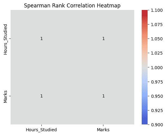
Step 3: Visualizing Spearman Correlation
- Heatmap displays correlation between only the selected columns
- Helps visually confirm strength of relationship
corr_data = df[['Hours_Studied', 'Marks']].corr(method='spearman')

sns.heatmap(corr_data, annot=True, cmap='coolwarm')
plt.title("Spearman Rank Correlation Heatmap")
plt.show()
Output:
Step 4: Scatter Plot for Monotonic Relationship
plt.scatter(df['Hours_Studied'], df['Marks'])
plt.xlabel("Hours Studied")
plt.ylabel("Marks")
plt.title("Monotonic Relationship")
plt.show()
Output:
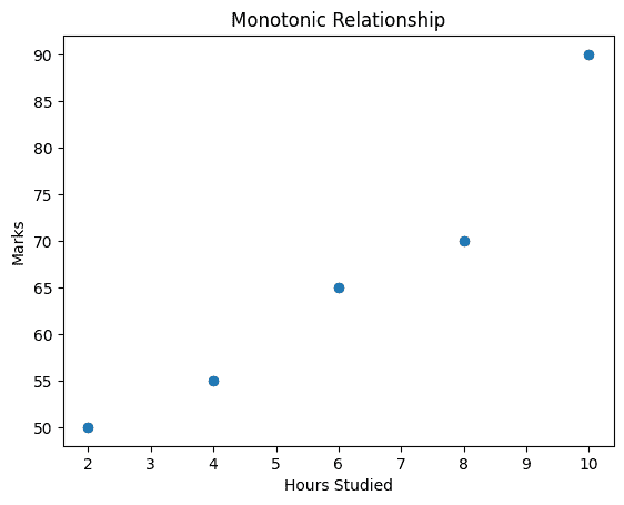
Scatter plot shows consistent upward trend hence confirming monotonic relationship.
Difference Between Pearson and Spearman Correlation
Lets see difference between Pearson Correlation and Spearman Correlation:
| Aspect | Pearson Correlation | Spearman Correlation |
|---|---|---|
| Data type | Continuous | Ordinal or continuous |
| Uses actual values | Yes | No |
| Uses ranks | No | Yes |
| Assumes normal distribution | Yes | No |
| Relationship type | Linear | Monotonic |
Advantages
- Works with non-linear monotonic data
- Less affected by outliers
- Simple to compute and interpret
- No strict distribution assumptions
Limitations
- Ignores actual data values
- Cannot detect non-monotonic patterns
- Less informative for precise numerical relationships
- Less accurate for very small datasets
Applications
- Ranking students based on marks
- Comparing search result rankings
- Measuring customer satisfaction levels
- Behavioral and social science studies
- Survey data analysis
- Feature ranking in ML
- Medical and social science studies