Detect and Remove the Outliers using Python

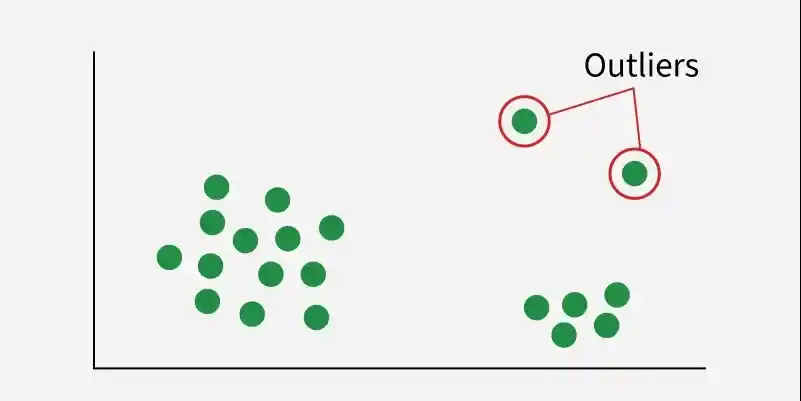
Outliers are data points that are very different from most other values in a dataset. They can occur due to measurement errors, unusual events or natural variation in the data. If not handled properly, they can affect analysis results and reduce machine learning model performance.

Detecting and Removing Outliers

There are several ways to detect and handle outliers in Python. We can use visualization methods or statistical techniques depending on the type of data. In this section, we will use Pandas and Matplotlib on the Diabetes dataset, which is available in the Scikit-learn library.

1. Visualizing and Removing Outliers Using Box Plots

A box plot helps visualize how data is distributed using quartiles. Any points outside the whiskers of the box plot are considered outliers. It is a simple way to see where most data values lie and identify unusual values.

import sklearn
from sklearn.datasets import load_diabetes
import pandas as pd
import seaborn as sns
import matplotlib.pyplot as plt

diabetes = load_diabetes()

column_name = diabetes.feature_names
df_diabetics = pd.DataFrame(diabetes.data, columns=column_name)

sns.boxplot(x=df_diabetics['bmi'])
plt.title('Boxplot of BMI')
plt.show()

Output:

In a box plot, outliers appear as points outside the whiskers. These values are much higher or lower than most of the data. For example, BMI values above 0.12 may be considered outliers

Removing Outliers

To remove outliers, we can define a threshold value and filter the data.

def removal_box_plot(df, column, threshold):
    removed_outliers = df[df[column] <= threshold]

    sns.boxplot(removed_outliers[column])
    plt.title(f'Box Plot without Outliers of {column}')
    plt.show()
    return removed_outliers

threshold_value = 0.12

no_outliers = removal_box_plot(df_diabetics, 'bmi', threshold_value)

Output:

2. Visualizing and Removing Outliers Using Scatter Plots

Scatter plots help show the relationship between two variables. They are useful when working with paired numerical data. In a scatter plot, outliers appear as points that are far away from the main group of data points.

fig, ax = plt.subplots(figsize=(6, 4))
ax.scatter(df_diabetics['bmi'], df_diabetics['bp'])
ax.set_xlabel('BMI')
ax.set_ylabel('Blood Pressure')
plt.title('Scatter Plot of BMI vs Blood Pressure')
plt.show()

Output:

From the graph, most data points are grouped in the bottom left corner. However, a few points appear in the opposite area, the top right corner of the graph. These points can be considered outliers because they are far from the main cluster of data.

Removing Outliers

• np.where(): Used to find the positions (indices) in the DataFrame where a condition is true.
• (df_diabetics['bmi'] > 0.12) and (df_diabetics['bp'] < 0.8): This condition identifies outliers where bmi is greater than 0.12 and bp is less than 0.8.

import numpy as np
import seaborn as sns
import matplotlib.pyplot as plt

outlier_indices = np.where((df_diabetics['bmi'] > 0.12) & (df_diabetics['bp'] < 0.8))

no_outliers = df_diabetics.drop(outlier_indices[0])

fig, ax_no_outliers = plt.subplots(figsize=(6, 4))
ax_no_outliers.scatter(no_outliers['bmi'], no_outliers['bp'])
ax_no_outliers.set_xlabel('(body mass index of people)')
ax_no_outliers.set_ylabel('(bp of the people )')
plt.show()

Output:

This removes rows where BMI > 0.12 and BP < 0.8 conditions derived from visual inspection.

3. Z-Score Method for Outlier Detection

The Z-score, also called the standard score, shows how far a data point is from the mean in terms of standard deviations. If the Z-score is greater than a chosen threshold , the value is considered an outlier.

• Z-scores are calculated for the 'age' column in df_diabetics.
• The zscore() function from SciPy stats is used.
• The result z shows how far each value is from the mean in standard deviations.

from scipy import stats
import numpy as np
z = np.abs(stats.zscore(df_diabetics['age']))
print(z)

Output:

An outlier threshold is usually set to 3.0. This is because about 99.7% of data points in a normal (Gaussian) distribution lie within \pm3 standard deviations from the mean.

Removing Outliers: Trimming and Capping

After identifying outliers using the Z-score method, we can handle them in two common ways: trimming or capping.

• Trimming removes the rows that contain outliers from the dataset.
• Capping keeps the rows but replaces extreme values with a predefined limit.

Trimming Outliers

import numpy as np

threshold_z = 2

outlier_indices = np.where(z > threshold_z)[0]
no_outliers = df_diabetics.drop(outlier_indices)

print("Original DataFrame Shape:", df_diabetics.shape)
print("DataFrame Shape after Removing Outliers:", no_outliers.shape)

Output:

Original DataFrame Shape: (442, 10)
DataFrame Shape after Removing Outliers: (426, 10)

Capping Outliers

threshold_z = 2

df_capped = df_diabetics.copy()

df_capped['age'] = np.where(z > threshold_z,
                            df_diabetics['age'].mean() + threshold_z * df_diabetics['age'].std(),
                            df_diabetics['age'])

print("Original DataFrame Shape:", df_diabetics.shape)
print("DataFrame Shape after Capping Outliers:", df_capped.shape)

Output:

Original DataFrame Shape: (442, 10)

DataFrame Shape after Capping Outliers: (442, 10)

4. Interquartile Range (IQR) Method

The IQR (Interquartile Range) method is a common and reliable technique for detecting outliers. It works well even when the data is skewed and identifies extreme values using quartiles. The IQR is calculated as the difference between the third quartile (Q3) and the first quartile (Q1):

IQR = Q3 - Q1

Here, we calculate the IQR for the 'bmi' column in df_diabetics. First Q1 and Q3 are found, then IQR = Q3 − Q1, which shows the spread of the middle 50% of the data.

Q1 = np.percentile(df_diabetics['bmi'], 25, method='midpoint')
Q3 = np.percentile(df_diabetics['bmi'], 75, method='midpoint')
IQR = Q3 - Q1
print(IQR)

Output:

0.06520763046978838

To identify outliers, we define upper and lower limits using the IQR value. Any value outside this range is treated as an outlier.

• upper = Q3 +1.5*IQR
• lower = Q1 - 1.5*IQR

upper = Q3+1.5*IQR
upper_array = np.array(df_diabetics['bmi'] >= upper)
print("Upper Bound:", upper)
print(upper_array.sum())

lower = Q1-1.5*IQR
lower_array = np.array(df_diabetics['bmi'] <= lower)
print("Lower Bound:", lower)
print(lower_array.sum())

Output:

Removing Outliers: Trimming and Capping

Trimming Outliers

import numpy as np
import sklearn
from sklearn.datasets import load_diabetes
import pandas as pd

diabetes = load_diabetes()

column_name = diabetes.feature_names
df_diabetes = pd.DataFrame(diabetes.data)
df_diabetes.columns = column_name

print("Old Shape:", df_diabetes.shape)

Q1 = df_diabetes['bmi'].quantile(0.25)
Q3 = df_diabetes['bmi'].quantile(0.75)
IQR = Q3 - Q1

lower = Q1 - 1.5 * IQR
upper = Q3 + 1.5 * IQR

upper_array = np.where(df_diabetes['bmi'] >= upper)[0]
lower_array = np.where(df_diabetes['bmi'] <= lower)[0]

df_diabetes.drop(index=upper_array, inplace=True)
df_diabetes.drop(index=lower_array, inplace=True)

print("New Shape:", df_diabetes.shape)

Output:

Old Shape: (442, 10)
New Shape: (439, 10)

Capping Outliers

df_capped = df_diabetes.copy()

df_capped['bmi'] = np.where(df_capped['bmi'] > upper, upper, df_capped['bmi'])
df_capped['bmi'] = np.where(df_capped['bmi'] < lower, lower, df_capped['bmi'])

print("Shape after Capping:", df_capped.shape)

Output:

Shape after Capping: (439, 10)

Download full code from here.